docker(28) Openjij チュートリアルをdockerで

実行手順

docker起動。masOSとなっているが、Windows, Linuxでも、/Users/administrator/openjij/workを、実際にホスト側で存在するフォルダ名にすればよい。

まずは第１章を実行したものをdocker hubに登録。
次の実行手順で実行できるはず。ただし、-p の後のポート番号は他のdocker等が使っていない番号にする。

macOS

$ docker run -p 8080:8080 -v /Users/administrator/openjij/work:/openjij/work -it kaizenjapan/openjij-ch1-ubuntu /bin/bash 

ただし、ユーザ名がAdministratorで、openjij/workフォルダが作ってある場合。

dockerでは、

root@f85c350c3f1e:/# cd openjij
root@f85c350c3f1e:/openjij# ls
ch1  work
root@f85c350c3f1e:/openjij# ls ch1
ch1.png  ising.py  openjij-ch1g.py  openjij-ch1gu.py
root@f85c350c3f1e:/openjij# cd ch1
root@f85c350c3f1e:/openjij/ch1# python3 openjij-ch1gu.py

で実行できる。

# cp ch1.png ../work

すれば、ホスト側のworkファイルにpngファイルがコピーできる。

#説明
Openjijをdockerで(追試)
https://qiita.com/kaizen_nagoya/items/ec1f7b1dbb64e5e22f7f
の後で実行した命令。

ubuntu

# pip install matplotlib

OpenJij チュートリアル
https://openjij.github.io/OpenJijTutorial/_build/html/ja/index.html

#第１章

openjij-ch1.py

import openjij as oj
#https://openjij.github.io/OpenJijTutorial/_build/html/ja/index.html
import numpy as np
import matplotlib.pyplot as plt

# 問題を表す縦磁場と相互作用を作ります。OpenJijでは辞書型で問題を受け付けます。
N = 5
h = {i: -1 for i in range(N)}
J = {(i, j): -1 for i in range(N) for j in range(i+1, N)}

print('h_i: ', h)
print('Jij: ', J)

# まず問題を解いてくれるSamplerのインスタンスを作ります。このインスタンスの選択で問題を解くアルゴリズムを選択できます。
sampler = oj.SASampler()
# samplerのメソッドに問題(h, J)を投げて問題を解きます。
response = sampler.sample_ising(h, J)

# 計算した結果(状態)は result.states に入っています。
print(response.states)

# もしくは添字付きでみるには samples を見ます。
print(response.samples)

# 実は h, J の添字を示す、辞書のkeyは数値以外も扱えます。
h = {'a': -1, 'b': -1}
J = {('a', 'b'): -1, ('b', 'c'): 1}
sampler = oj.SASampler(iteration=10)  # 10回 SAで解いてみる. iteration という引数で10回分一気に解くことができます。
response = sampler.sample_ising(h, J)
print(response.states)

print(response.energies)

print(response.indices)

print(response.samples)

print(response.min_samples)

# Q_ij を辞書型でつくります。
Q = {(0, 0): -1, (0, 1): -1, (1, 2): 1, (2, 2): 1}
sampler = oj.SASampler(iteration=3)
# QUBOを解く時は .sample_qubo を使いましょう
response = sampler.sample_qubo(Q)
print(response.states)

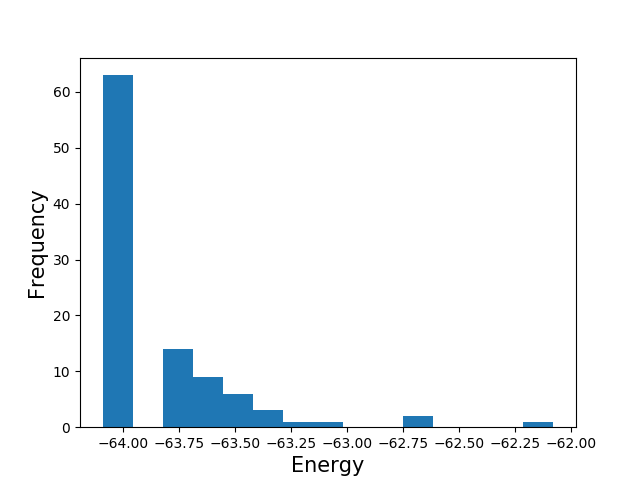
N = 50
# ランダムにQij を作る
import random
Q = {(i, j): random.uniform(-1, 1) for i in range(N) for j in range(i+1, N)}

# OpenJijで解く
sampler = oj.SASampler(iteration=100)
response = sampler.sample_qubo(Q)

# エネルギーを少しみてみます。
print(response.energies[:5])


plt.hist(response.energies, bins=15)
plt.xlabel('Energy', fontsize=15)
plt.ylabel('Frequency', fontsize=15)
plt.show()

min_samples = response.min_samples

print(min_samples)

pythonで実行し、出力するようにprint関数を追記している。
実行すると

# python3 openjij-ch1.py
h_i:  {0: -1, 1: -1, 2: -1, 3: -1, 4: -1}
Jij:  {(0, 1): -1, (0, 2): -1, (0, 3): -1, (0, 4): -1, (1, 2): -1, (1, 3): -1, (1, 4): -1, (2, 3): -1, (2, 4): -1, (3, 4): -1}
[[1, 1, 1, 1, 1]]
[{0: 1, 1: 1, 2: 1, 3: 1, 4: 1}]
[[1, 1, -1], [1, 1, -1], [1, 1, -1], [1, 1, -1], [1, 1, -1], [1, 1, -1], [1, 1, -1], [1, 1, -1], [1, 1, -1], [1, 1, -1]]
[-4.0, -4.0, -4.0, -4.0, -4.0, -4.0, -4.0, -4.0, -4.0, -4.0]
['a', 'b', 'c']
[{'a': 1, 'b': 1, 'c': -1}, {'a': 1, 'b': 1, 'c': -1}, {'a': 1, 'b': 1, 'c': -1}, {'a': 1, 'b': 1, 'c': -1}, {'a': 1, 'b': 1, 'c': -1}, {'a': 1, 'b': 1, 'c': -1}, {'a': 1, 'b': 1, 'c': -1}, {'a': 1, 'b': 1, 'c': -1}, {'a': 1, 'b': 1, 'c': -1}, {'a': 1, 'b': 1, 'c': -1}]
{'min_states': array([[ 1,  1, -1]]), 'num_occurrences': array([10]), 'min_energy': -4.0}
[[1, 1, 0], [1, 1, 0], [1, 1, 0]]
[-61.12030947336661, -61.12030947336661, -61.12030947336661, -61.12030947336661, -61.12030947336661]
{'min_states': array([[1, 0, 1, 1, 0, 1, 0, 0, 1, 0, 1, 1, 0, 1, 1, 1, 0, 0, 1, 0, 0, 0,
        1, 0, 1, 1, 1, 1, 1, 0, 0, 1, 1, 1, 1, 0, 0, 1, 0, 1, 0, 0, 0, 0,
        1, 0, 1, 1, 1, 1]]), 'num_occurrences': array([68]), 'min_energy': -61.12030947336661}

グラフが出ない。少し加筆。

dockerで機械学習(1) with anaconda(1)「ゼロから作るDeep Learning - Pythonで学ぶディープラーニングの理論と実装」斎藤 康毅 著
https://qiita.com/kaizen_nagoya/items/a7e94ef6dca128d035ab

ではファイル出力にした。同様にしようとすれば、

pythonファイル編集

1. PNGファイル出力のおまじない:２行追記

import matplotlib as mpl
mpl.use('Agg')

1. ファイル出力操作：２行追記、１行注釈化

fig = plt.figure()
#plt.show()
fig.savefig('ch1.png')

結果はch1.pngファイルとして出力

課題は、文字コード。

量子計算機　arXiv掲載　西森 秀稔　論文単語帳作成をdockerで（文字コード対応）
https://qiita.com/kaizen_nagoya/items/319672853519990cee42
に記録した方法で変換

ubuntu

# apt -y install n/f
# nkf -w openjij-ch1g.py > openjij-ch1gu.py

#第２章

openjij-ch2.py

import random
import numpy as np
import matplotlib.pyplot as plt
import openjij as oj

# 反強磁性1次元イジングモデル を作る.
N = 30
h = {0: -10}
J = {(i, i+1): 1 for i in range(N-1)}

# 最適解
correct_state = [(-1)**i for i in range(N)]

# TTS を計算するのに必要なp^R
pR = 0.99

# Samplerの引数のstep_num というパラメータに渡すリスト(step_num_list)
# step_num はアニーリング中のパラメータ(温度, 横磁場)を下げていくときの分割数
# なので増やせば増やすほどゆっくりアニーリングすることになってアニーリング時間が伸びる。
step_num_list = [10, 20, 30, 40]

# 各計算時間に対するTTSを格納しておくリスト
TTS_list = []
tau_list = []  # 計算時間を格納しておくリスト

iteration = 2000  # 確率を計算するために1回のアニーリングを行う回数

for step_num in step_num_list:
    # beta_max と　beta_min はSAのアルゴリズムで使うパラメータ.
    # 確率p_sを計算するために500回計算する
    sampler = oj.SASampler(beta_max=10.0, beta_min=0.01, step_num=step_num, iteration=iteration)

    response = sampler.sample_ising(h, J)
    # 返ってきた解であっている状態の数を数えて最適解を得た確率を計算する。
    tau = response.info['execution_time']
    ps = sum([1 if state == correct_state else 0 for state in response.states])/iteration

    # ps=0だとTTSが無限大になってしまうのでそこは回避
    if ps == 0:
        continue

    # TTSを計算する
    TTS_list.append(np.log(1-pR)/np.log(1-ps)*tau)
    tau_list.append(tau)

plt.plot(tau_list, TTS_list)
plt.xlabel('annealing time')
plt.ylabel('TTS')

result = oj.benchmark(
                      true_ground_states=[correct_state], ground_energy=0,
                      solver= lambda time_param, iteration: oj.SASampler(step_num=time_param, iteration=iteration).sample_ising(h,J),
                      time_param_list=step_num_list,
                      p_d=0.99
            )
fig, (axL,axC,axR) = plt.subplots(ncols=3, figsize=(15,3))
plt.subplots_adjust(wspace=0.4)

fontsize = 10
axL.plot(result['time'], result['tts'])
axL.set_xlabel('annealing time', fontsize=fontsize)
axL.set_ylabel('TTS', fontsize=fontsize)

axC.plot(result['time'], result['e_res'])
axC.set_xlabel('annealing time', fontsize=fontsize)
axC.set_ylabel('Residual energy', fontsize=fontsize)

axR.plot(result['time'], result['error'])
axR.set_xlabel('annealing time', fontsize=fontsize)
axR.set_ylabel('Error probability', fontsize=fontsize)

fig.show()

import time
def anti_ferro_solver(time_param, iteration, h, J):
    """
    すべて 1 と [1,-1,1,...] と [-1,1,-1,...] の3つの状態からランダムに選ぶ
    """

    # 入力された h と J から添字の集合をつくる
    indices = set(h.keys())
    indices = list(indices | set([key for keys in J.keys() for key in keys]))

    ones_state = list(np.ones(len(indices), dtype=int))        # all 1

    minus_plus_state = np.ones(len(indices), dtype=int)
    minus_plus_state[::2] *= -1                                         # -1, 1, -1, 1, ...
    plus_minus_state = -1 * minus_plus_state                   # 1, -1, 1, -1

    start = time.time()
    _states = [ones_state, list(minus_plus_state), list(plus_minus_state)]
    state_record = [_states[np.random.randint(3)] for _ in range(iteration)]   # 3つの状態からランダムにひとつ選ぶ
    exec_time = (time.time()-start) * 10**6 * time_param                                # 適当に計算時間を伸ばしておきます

    energies = [sum(state) for state in state_record]                                     # エネルギーの計算はてきとうです


    # Responseクラスに状態とエネルギーを格納します
    response = oj.Response(indices=indices, var_type='SPIN')
    response.update_ising_states_energies(state_record, energies)
    response.info['execution_time'] = exec_time

    return response

result = oj.benchmark(
                      true_ground_states=[correct_state], ground_energy=0,
                      solver= lambda time_param, iteration: anti_ferro_solver(time_param, iteration, h, J),
                      time_param_list=step_num_list,
                      iteration=100,
                      p_d=0.99
            )

fig, (axL,axC,axR) = plt.subplots(ncols=3, figsize=(15,3))
plt.subplots_adjust(wspace=0.4)

fontsize = 10
axL.plot(result['time'], result['tts'])
axL.set_xlabel('annealing time', fontsize=fontsize)
axL.set_ylabel('TTS', fontsize=fontsize)

axC.plot(result['time'], result['e_res'])
axC.set_xlabel('annealing time', fontsize=fontsize)
axC.set_ylabel('Residual energy', fontsize=fontsize)

axR.plot(result['time'], result['error'])
axR.set_xlabel('annealing time', fontsize=fontsize)
axR.set_ylabel('Error probability', fontsize=fontsize)

fig.show()

[7]がみあたらない。なぜかエラーが出てる。下記記事で調査中。

python error collection
https://qiita.com/kaizen_nagoya/items/4b13c6c9574c44931943

#docker hub登録

macOS

$ docker commit 2651e9e533e2 kaizenjapan/openjij-ch1-ubuntu
sha256:31f8ffbbbf06db1691bd5386f547f553151cbfdd1cfff171e5dcec3eeed4d546
$ docker push kaizenjapan/openjij-ch1-ubuntu
The push refers to repository [docker.io/kaizenjapan/openjij-ch1-ubuntu]
42cc7cd900d4: Pushed 
75e70aa52609: Mounted from kaizenjapan/qc-nakamori 
dda151859818: Mounted from kaizenjapan/qc-nakamori 
fbd2732ad777: Mounted from kaizenjapan/qc-nakamori 
ba9de9d8475e: Mounted from kaizenjapan/qc-nakamori 
latest: digest: sha256:444a72af2904226c0a37adf6f7ff562398ed88a269ef3acba5f9efc6e3389647 size: 1365

参考資料(reference)

Dockerでホストとコンテナ間でのファイルコピー
https://qiita.com/gologo13/items/7e4e404af80377b48fd5

openjij slack
https://openjij.slack.com

!pip install -U cmake

文書履歴(document history)

ver. 0.01 初稿 20190626 朝
ver. 0.02 ファイル出力追記 20190626 午前
ver. 0.03 docker hub登録 20190626 昼
ver. 0.04 ch2書き掛け。20190626 午後
ver. 0.05 誤植訂正 20190626 夕

最後までおよみいただきありがとうございました。

いいね　💚、フォローをお願いします。

Thank you very much for reading to the last sentence.

Please press the like icon 💚　and follow me for your happy life.

https://b.hatena.ne.jp/guide/bbutton