前回
筑波大学の機械学習講座：課題のPythonスクリプト部分を作りながらsklearnを勉強する (13)
https://github.com/legacyworld/sklearn-basic

課題 6.4 ロジスティック回帰による予測

今回は初めてscikit-learnを使用しなかった。
Youtubeでの解説は第7回(1) 25分50秒あたり
問題としては難しくはないが、一つ注意点。

w^T = (w_0,w_1,w_2),
X = \begin{pmatrix}
x_{11}&x_{12}&\cdots&x_{110} \\
x_{21}&x_{22}&\cdots&x_{210} \\
1&1&\cdots&1
\end{pmatrix} \\
w^TX = 0はx_1,x_2の平面上でw_0x_1 + w_1x_2 + w_2 = 0と表される。変形して\\
x_2 = -\frac{w_2}{w_1} - \frac{w_0}{w_1}x_1

普通は$w_0$が切片部分になるのだが、この問題では$w_2$になっている。
ソースコードはこちら

Homework_6.4.py

import numpy as np
import matplotlib.pyplot as plt
# シグモイド関数
def sigmoid(w,x):
    return 1/(1+np.exp(-np.dot(w,x)))

# 0.5で分類
def classification(a):
    return 1 if a > 0.5 else 0

X = np.array([[1.5,-0.5],[-0.5,-1.0],[1.0,-2.5],[1.5,-1.0],[0.5,0.0],[1.5,-2.0],[-0.5,-0.5],[1.0,-1.0],[0.0,-1.0],[0.0,0.5]])
# 切片部分が後ろに来ているので、1を最後に追加
X = np.concatenate([X,np.ones(10).reshape(-1,1)],1)
y = np.array([1,0,0,1,1,1,0,1,0,0])
w = np.array([[6,3,-2],[4.6,1,-2.2],[1,-1,-2]])
# 解説と同じ参考用のロジット等高線作成
fig = plt.figure(figsize=(20,10))
ax = [fig.add_subplot(2,2,i+1) for i in range(4)]
ax[0].scatter(X[:,0],X[:,1])
x_plot = np.linspace(-1.0,2.0,100)
ax[0].set_ylim(-3,1)
for i in range(0,3,1):
    y_plot = -w[i][2]/w[i][1]-w[i][0]/w[i][1]*x_plot
    ax[0].plot(x_plot,y_plot,label=f"w{i+1}")
ax[0].set_title("Sample Distribution")
ax[0].legend()
ax[0].grid(b=True)

# メッシュデータ
xlim = [-2.0,2.0]
ylim = [-3.0,3.0]
n = 100
xx = np.linspace(xlim[0], xlim[1], n)
yy = np.linspace(ylim[0], ylim[1], n)
YY, XX = np.meshgrid(yy, xx)
xy = np.vstack([XX.ravel(), YY.ravel(),np.ones(n**2)])

for i in range(3):
    Z = sigmoid(w[i],xy).reshape(XX.shape)
    interval = np.arange(0,1,0.01)
    # 0が紫、1が赤、その間をグラデーション
    m = ax[i+1].contourf(XX,YY,Z,interval,cmap="rainbow",extend="both")
    m = ax[i+1].scatter(X[:,0],X[:,1],c=y)
    ax[i+1].set_title(f"w{i+1} Logit Contour")
    fig.colorbar(mappable = m,ax=ax[i+1])
plt.savefig("6.4.png")

# w^T x の計算
for index,w_i in enumerate(w):
    print(f"w{index+1} {np.dot(w_i,X.T)}")

# sigmoid(w^T x)の計算
np.set_printoptions(formatter={'float': '{:.2e}'.format})
for index,w_i in enumerate(w):
    print(f"w{index+1} {sigmoid(w_i,X.T)}")

# 分類
for index,w_i in enumerate(w):
    print(f"w{index+1} {np.vectorize(classification)(sigmoid(w_i,X.T))}")

# 確率
for index,w_i in enumerate(w):
    print(f"w{index+1} {np.count_nonzero(np.vectorize(classification)(sigmoid(w_i,X.T))==y)*10}%")

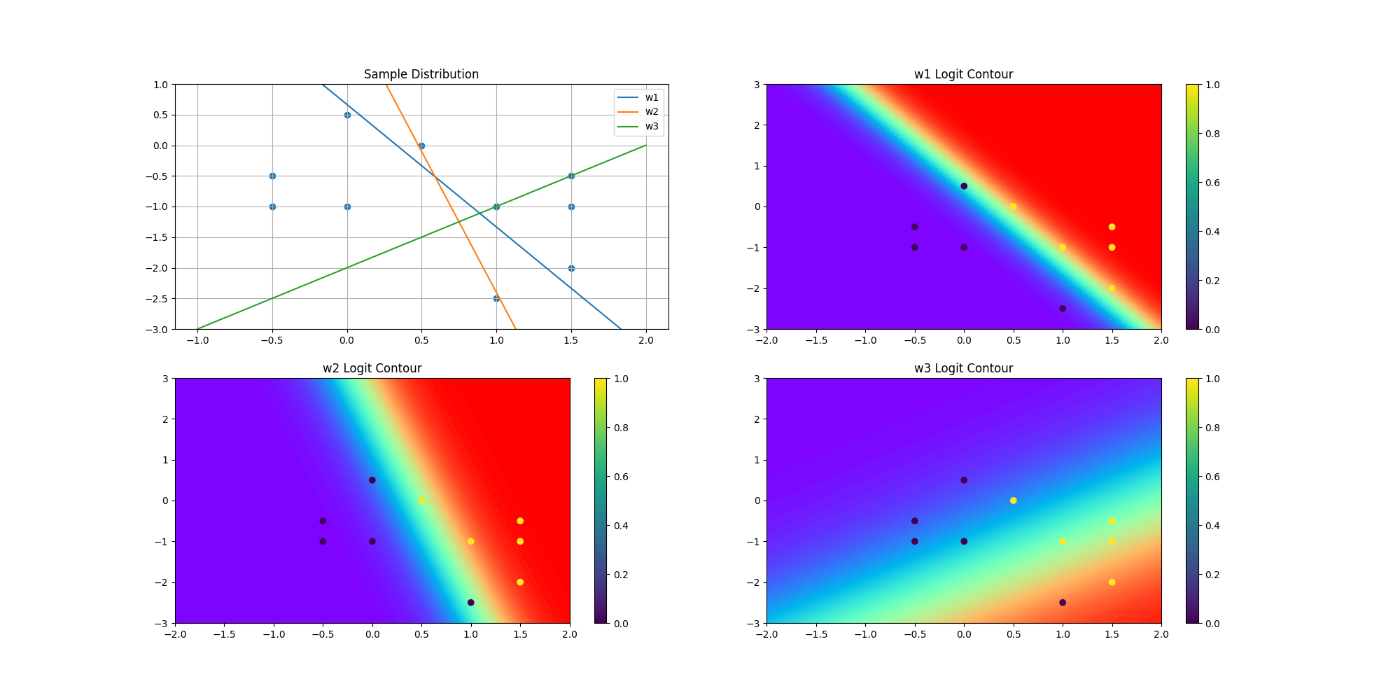
解説で見せているロジット等高線はこれ。

実行結果はこちら

$w_i^Tx_j (i=1,2,3 j=1,2,...,10)$

w1 [ 5.5 -8.  -3.5  4.   1.   1.  -6.5  1.  -5.  -0.5]
w2 [ 4.2 -5.5 -0.1  3.7  0.1  2.7 -5.   1.4 -3.2 -1.7]
w3 [ 0.  -1.5  1.5  0.5 -1.5  1.5 -2.   0.  -1.  -2.5]

$\sigma(w_i^Tx_j) (i=1,2,3 j=1,2,...,10)$

w1 [9.96e-01 3.35e-04 2.93e-02 9.82e-01 7.31e-01 7.31e-01 1.50e-03 7.31e-01 6.69e-03 3.78e-01]
w2 [9.85e-01 4.07e-03 4.75e-01 9.76e-01 5.25e-01 9.37e-01 6.69e-03 8.02e-01 3.92e-02 1.54e-01]
w3 [5.00e-01 1.82e-01 8.18e-01 6.22e-01 1.82e-01 8.18e-01 1.19e-01 5.00e-01 2.69e-01 7.59e-02]

$モデル\sigma(w_i^Tx_j)によるx_jの分類結果$

w1 [1 0 0 1 1 1 0 1 0 0]
w2 [1 0 0 1 1 1 0 1 0 0]
w3 [0 0 1 1 0 1 0 0 0 0]

正解率

w1 100%
w2 100%
w3 60%

過去の投稿

筑波大学の機械学習講座：課題のPythonスクリプト部分を作りながらsklearnを勉強する (14)

課題 6.4 ロジスティック回帰による予測

過去の投稿