前回からの続き
筑波大学の機械学習講座：課題のPythonスクリプト部分を作りながらsklearnを勉強する (1)
https://github.com/legacyworld/sklearn-basic

課題 3.1 多項式回帰の二乗誤差

これは$y = \sin(x)$に$N(0,1)\times0.1$の誤差を載せた訓練データを作り、それを多項式で回帰させる問題。
解説は第3回(1) 56分40秒あたり

Homework_3.1.py

import pandas as pd
import numpy as np
import matplotlib.pyplot as plt
import copy
from sklearn.preprocessing import PolynomialFeatures as PF
from sklearn import linear_model
from sklearn.metrics import mean_squared_error
# 訓練用データの数
NUM_TR = 6
np.random.seed(0)
rng = np.random.RandomState(0)

# 描画用のx軸データ
x_plot = np.linspace(0,10,100)
# 訓練データ
tmp = copy.deepcopy(x_plot)
rng.shuffle(tmp)
x_tr = np.sort(tmp[:NUM_TR])
y_tr = np.sin(x_tr) + 0.1*np.random.randn(NUM_TR)

# Matrixへ変換
X_tr = x_tr.reshape(-1,1)
X_plot = x_plot.reshape(-1,1)

# 多項式用のデータ
# 次数決め打ち
degree = 1
pf = PF(degree=degree)
X_poly = pf.fit_transform(X_tr)
X_plot_poly = pf.fit_transform(X_plot)

model = linear_model.LinearRegression()
model.fit(X_poly,y_tr)
fig = plt.figure()
plt.scatter(x_tr,y_tr,label="training Samples")
plt.plot(x_plot,model.predict(X_plot_poly),label=f"degree = {degree}")
plt.legend()
plt.ylim(-2,2)
fig.savefig(f"{degree}.png")

# 多項式用のデータ
# 全ての次数
fig = plt.figure()
plt.scatter(x_tr,y_tr,label="Training Samples")

for degree in range(1,NUM_TR):
    pf = PF(degree=degree)
    X_poly = pf.fit_transform(X_tr)
    X_plot_poly = pf.fit_transform(X_plot)
    model = linear_model.LinearRegression()
    model.fit(X_poly,y_tr)
    plt.plot(x_plot,model.predict(X_plot_poly),label=f"degree {degree}")
    plt.legend()
    mse = mean_squared_error(y_tr,model.predict(X_poly))
    print(f"degree = {degree} mse = {mse}")

plt.xlim(0,10)
plt.ylim(-2,2)
fig.savefig('all_degree.png')

回帰の計算をさせるためのデータ(x_tr)とグラフ描画用(x_plot)で2つ用意している。
単にx_tr = x_plotとやると実データがコピーされない。
そのままやるとx_tr = np.sort(tmp[:NUM_TR])の部分で描画用データの数もNUM_TRになってしまい、グラフ描画がおかしくなる。
なのでdeepcopyを利用している。

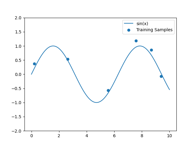
元データとして0-10の間を100等分したものを用意している。
訓練用データはそのうちNUM_TRだけランダムに選ぶ（講座では６つ）
誤差として0-1の間で発生させた乱数に1/10をかけたものをsin(x_tr)に足している。
最初にseedを固定しているため、どの環境で何回実行しても同じ結果が出る。
用意されたデータはこれ

これまでと異なるのはPolynomialFeaturesという部分である。
これは多項式の次数の分だけ$x,x^2,x^3,x^4$と訓練データを用意する部分になる。
例えば次数 = 3だとこうなる。

degree = 3
pf = PF(degree=degree)
X_poly = pf.fit_transform(X_tr)
print(f"degree = {degree}\nX_Tr = {X_tr}\nX_poly = {X_poly}")

実行結果は

degree = 3
X_Tr = [[0.2020202 ]
 [2.62626263]
 [5.55555556]
 [7.57575758]
 [8.68686869]
 [9.39393939]]
X_poly = [[1.00000000e+00 2.02020202e-01 4.08121620e-02 8.24488122e-03]
 [1.00000000e+00 2.62626263e+00 6.89725538e+00 1.81140040e+01]
 [1.00000000e+00 5.55555556e+00 3.08641975e+01 1.71467764e+02]
 [1.00000000e+00 7.57575758e+00 5.73921028e+01 4.34788658e+02]
 [1.00000000e+00 8.68686869e+00 7.54616876e+01 6.55525771e+02]
 [1.00000000e+00 9.39393939e+00 8.82460973e+01 8.28978490e+02]]

1番目のデータだと元の訓練データは$x = 2.020202\times10^{-1}$で、$x^2=4.08\times10^{-2}$となっている。
要は$x^2,x^3$を別の特徴量として扱うわけである。

次に1次（直線）で回帰させてみる。結果はこれ。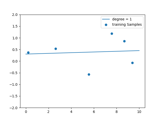

最後に次数を1-5で変化させてそれぞれグラフに描画してみる。

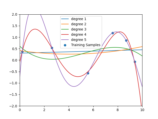
誤差はこれ。degree = 5だけ数字が合わなかった。

degree = 1 mse = 0.33075005001856256
degree = 2 mse = 0.3252271169458752
degree = 3 mse = 0.30290034474812344
degree = 4 mse = 0.010086018410257538
degree = 5 mse = 3.1604543144050787e-22

筑波大学の機械学習講座：課題のPythonスクリプト部分を作りながらsklearnを勉強する (2)

課題 3.1 多項式回帰の二乗誤差