More than 3 years have passed since last update.

筑波大学の機械学習講座：課題のPythonスクリプト部分を作りながらsklearnを勉強する (12)

Last updated at 2020-06-12Posted at 2020-06-11

前回
筑波大学の機械学習講座：課題のPythonスクリプト部分を作りながらsklearnを勉強する (11)
https://github.com/legacyworld/sklearn-basic

課題 6.2 カーネルとSVM

この課題は元データ(linear separation, moons, circles)のランダム値などがわからないため全く同じには出来なかったが、大体の傾向は掴めたと思う。
Youtubeでの解説：第7回(2) 48分30秒あたり

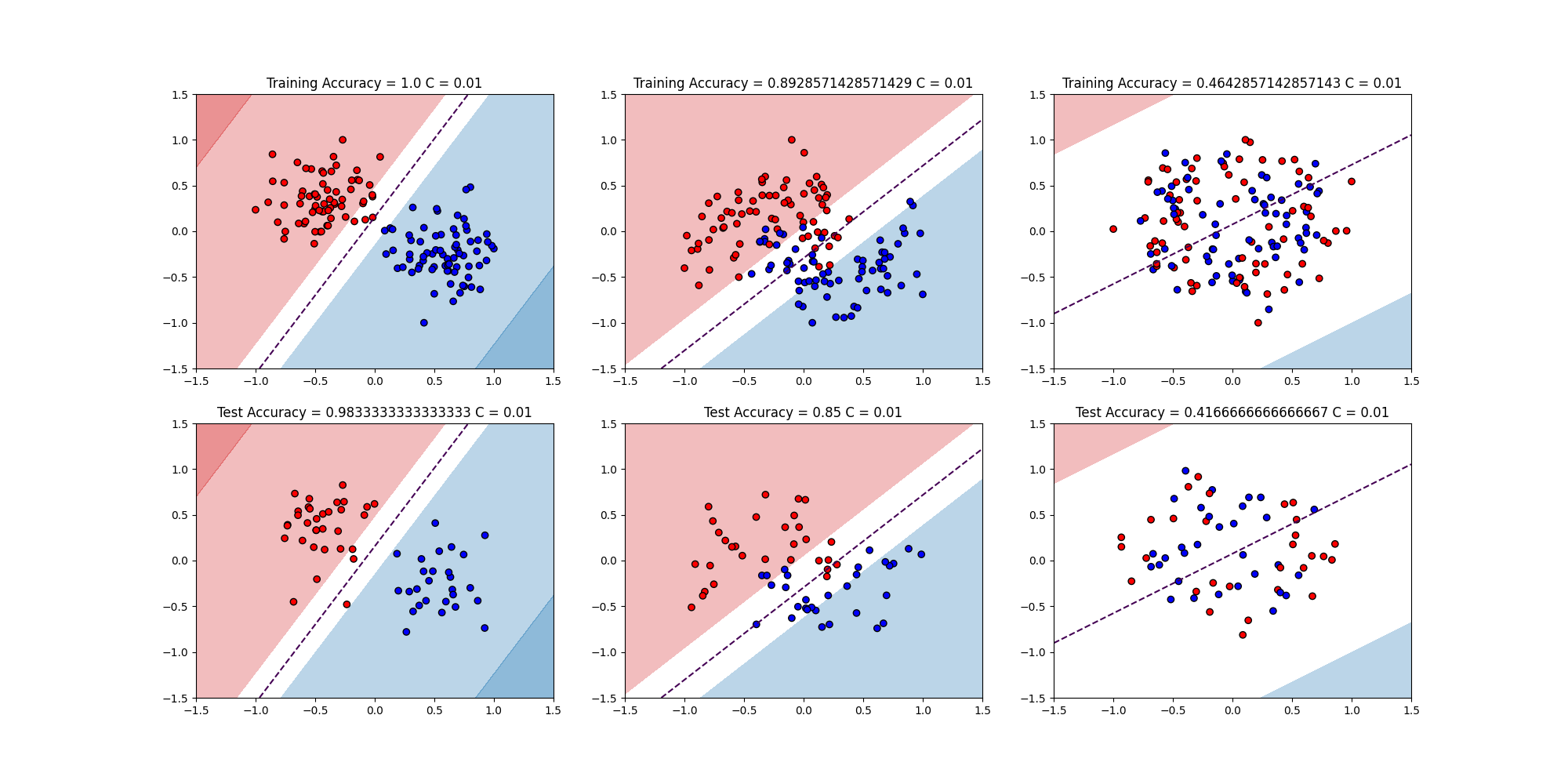
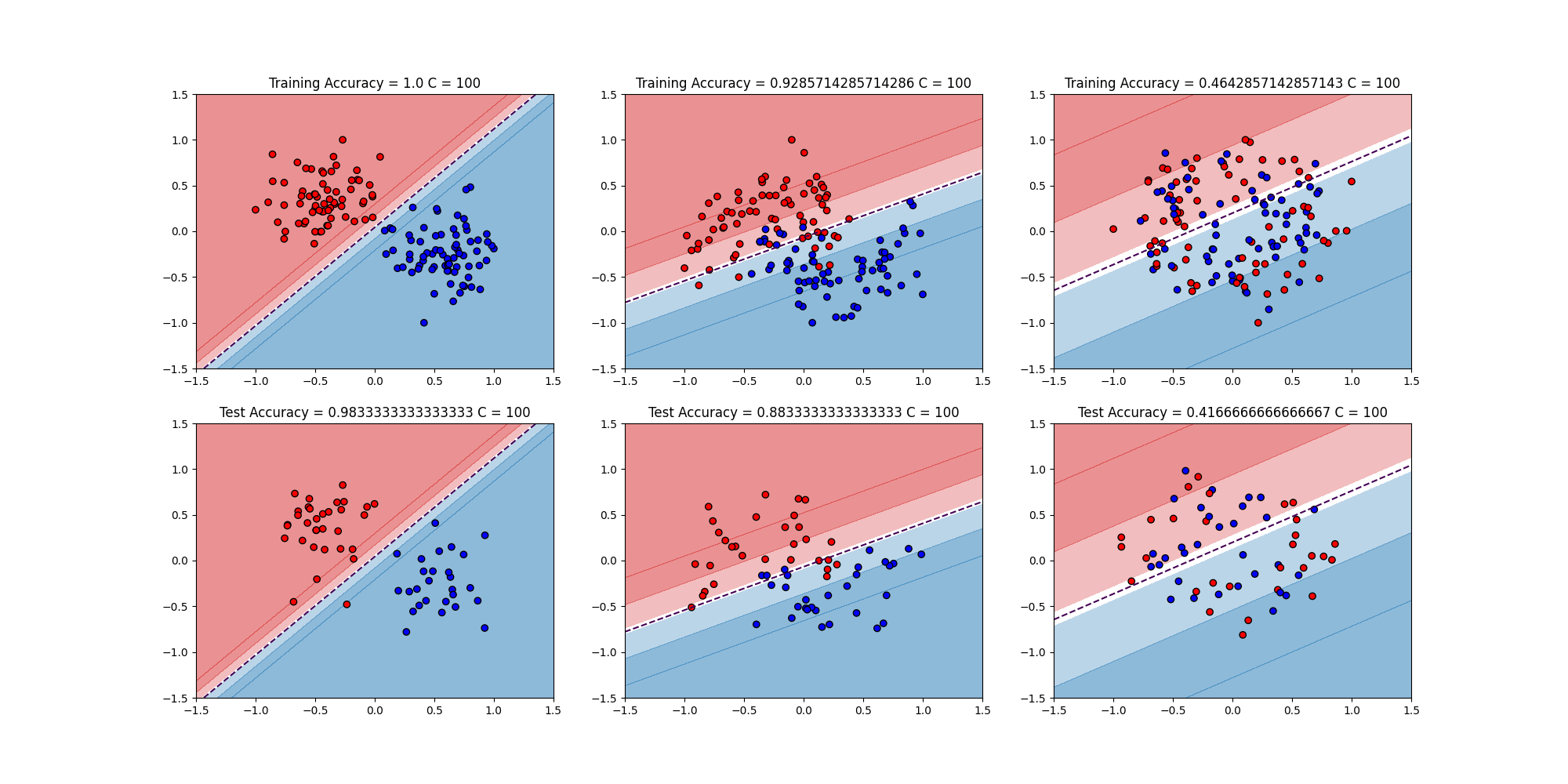
講義ではCの値を変えてもそんなに傾向は変わらないことを示している。その傾向とは

Linear Separation
- make_blobsで作ったデータなので綺麗に分類できる
moons
- 三日月が2つあわさった形なので綺麗に線形では分類は出来ないが、まぁまぁな結果
circles
- 円が2つ重なった状態なのでどうやっても線形では分類できない

$C = 0.01,0.1,0.5,1,10,100$で変えたものを全て画像に落とすプログラムとした。

Homework_6.2_linear.py

import numpy as np
import matplotlib.pyplot as plt
from matplotlib.colors import ListedColormap
import matplotlib.colors as mcolors
from sklearn import svm,metrics
from sklearn import preprocessing
from sklearn.model_selection import train_test_split
from sklearn.datasets import make_circles,make_moons,make_blobs

datanames = ['linear_separation','moons','circles']
samples = 200
c_values = [0.01,0.1,0.5,1,10,100]
# 3種類のデータ作成
def datasets(dataname):
    if dataname == 'linear_separation':
        X,y = make_blobs(n_samples=samples,centers=2,random_state=64)
    elif dataname == 'moons':
        X,y = make_moons(n_samples=samples,noise=0.3,random_state=74)
    elif dataname == 'circles':
        X,y = make_circles(n_samples=samples,noise=0.3,random_state=70)
    
    X = preprocessing.MinMaxScaler(feature_range=(-1,1)).fit_transform(X)
    return X,y
# Cとデータセットごとに分類を行う
def learn_test_plot(clf_models):
    for clf in clf_models:
        plt.clf()
        # 3種類のデータごとにTrain ErrorとTest Errorを描画（計6種類）
        fig = plt.figure(figsize=(20,10))
        ax = [fig.add_subplot(2,3,i+1) for i in range(6)]
        for a in ax:
            a.set_xlim(-1.5,1.5)
            a.set_ylim(-1.5,1.5)

        for dataname in datanames:
            X,y = datasets(dataname)
            X_tr_val,X_test,y_tr_val,y_test = train_test_split(X,y,test_size=0.3,random_state=42)
            X_tr,X_val,y_tr,y_val = train_test_split(X_tr_val,y_tr_val,test_size=0.2,random_state=42)
            clf.fit(X_tr,y_tr)
            dec = clf.decision_function(X_val)
            predict = clf.predict(X_val)
            train_acc = metrics.accuracy_score(y_val,predict)
            test_predict = clf.predict(X_test)
            test_acc = metrics.accuracy_score(y_test,test_predict)
            c_value = clf.get_params()['C']
            # メッシュデータ
            xlim = [-1.5,1.5]
            ylim = [-1.5,1.5]
            xx = np.linspace(xlim[0], xlim[1], 30)
            yy = np.linspace(ylim[0], ylim[1], 30)
            YY, XX = np.meshgrid(yy, xx)
            xy = np.vstack([XX.ravel(), YY.ravel()]).T
            Z = clf.decision_function(xy).reshape(XX.shape)
            # 塗りつぶし用の色
            blue_rgb = mcolors.to_rgb("tab:blue")
            red_rgb = mcolors.to_rgb("tab:red")
            # データセットごとに縦に並べる
            index = datanames.index(dataname)
            # decision_functionが大きいほど色を濃くする
            ax[index].contourf(XX, YY, Z,levels=[-2,-1,-0.1,0.1,1,2],colors=[red_rgb+(0.5,),red_rgb+(0.3,),(1,1,1),blue_rgb+(0.3,),blue_rgb+(0.5,)],extend='both')
            ax[index].contour(XX,YY,Z,levels=[0],linestyles=["--"])
            ax[index].scatter(X_tr_val[:,0],X_tr_val[:,1],c=y_tr_val,edgecolors='k',cmap=ListedColormap(['#FF0000','#0000FF']))
            ax[index].set_title(f"Training Accuracy = {train_acc} C = {c_value}")

            ax[index+3].contourf(XX, YY, Z,levels=[-2,-1,-0.1,0.1,1,2],colors=[red_rgb+(0.5,),red_rgb+(0.3,),(1,1,1),blue_rgb+(0.3,),blue_rgb+(0.5,)],extend='both')
            ax[index+3].contour(XX,YY,Z,levels=[0],linestyles=["--"])
            ax[index+3].scatter(X_test[:,0],X_test[:,1],c=y_test,edgecolors='k',cmap=ListedColormap(['#FF0000','#0000FF']))
            ax[index+3].set_title(f"Test Accuracy = {test_acc} C = {c_value}")

        plt.savefig(f"6.2_{c_value}.png")

clf_models = [svm.SVC(kernel='linear',C=c_value) for c_value in c_values]
learn_test_plot(clf_models)

$C = 0.01,1,100$の結果はこちら
まぁCを変えても同じ結果と言える

過去の投稿

You get articles that match your needs
You can efficiently read back useful information
You can use dark theme

What you can do with signing up