筑波大学の機械学習講座：課題のPythonスクリプト部分を作りながらsklearnを勉強する (1)
筑波大学の機械学習講座：課題のPythonスクリプト部分を作りながらsklearnを勉強する (2)
https://github.com/legacyworld/sklearn-basic

課題 3.2 多項式単回帰の訓練誤差とテスト誤差

Youtubeの解説は第4回(1) 40分あたり
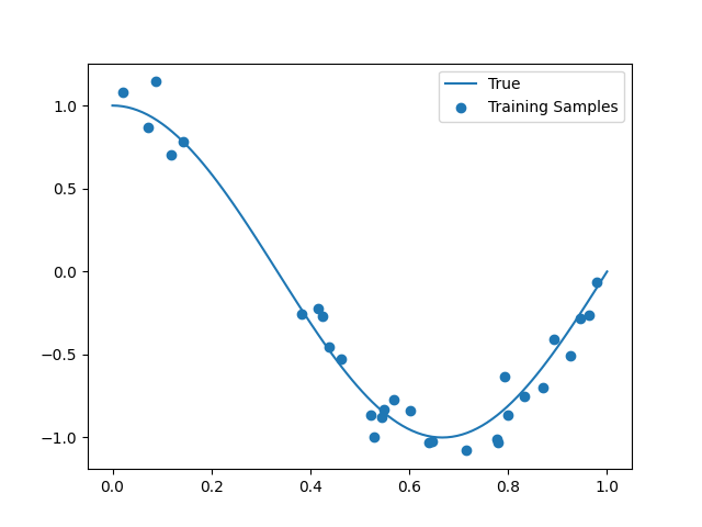
$y = \cos(1.5\pi x)$に$N(0,1)\times0.1$の誤差を載せた30個の訓練データを作り、多項式回帰を行う。
ここから交差検証が入る。
1次から20次まで順に回帰していく。
訓練データはこれ。

ソースコード

Homework_3.2.py

import pandas as pd
import numpy as np
import matplotlib.pyplot as plt
from sklearn.preprocessing import PolynomialFeatures as PF
from sklearn import linear_model
from sklearn.pipeline import Pipeline
from sklearn.metrics import mean_squared_error
from sklearn.model_selection import cross_val_score

DEGREE = 20

def true_f(x):
    return np.cos(1.5 * x * np.pi)

np.random.seed(0)
n_samples = 30

# 描画用のx軸データ
x_plot = np.linspace(0,1,100)
# 訓練データ
x_tr = np.sort(np.random.rand(n_samples))
y_tr = true_f(x_tr) + np.random.randn(n_samples) * 0.1
# Matrixへ変換
X_tr = x_tr.reshape(-1,1)
X_plot = x_plot.reshape(-1,1)

for degree in range(1,DEGREE+1):
    plt.scatter(x_tr,y_tr,label="Training Samples")
    plt.plot(x_plot,true_f(x_plot),label="True")
    plt.xlim(0,1)
    plt.ylim(-2,2)
    filename = f"{degree}.png"
    pf = PF(degree=degree,include_bias=False)
    linear_reg = linear_model.LinearRegression()
    steps = [("Polynomial_Features",pf),("Linear_Regression",linear_reg)]
    pipeline = Pipeline(steps=steps)
    pipeline.fit(X_tr,y_tr)
    plt.plot(x_plot,pipeline.predict(X_plot),label="Model")
    y_predict = pipeline.predict(X_tr)
    mse = mean_squared_error(y_tr,y_predict)
    scores = cross_val_score(pipeline,X_tr,y_tr,scoring="neg_mean_squared_error",cv=10)
    plt.title(f"Degree: {degree} TrainErr: {mse:.2e} TestErr: {-scores.mean():.2e}(+/- {scores.std():.2e})")
    plt.legend()
    plt.savefig(filename)
    plt.clf()

前回の課題3.1ではPolynomialFeaturesで$x,x^2,x^3$等を用意してから、LinearRegressionを行っていたが、pipelineというのを使うと一発で出来ることを学んだ。
実際に課題3.1の解説動画の中のソースコードを見るとpipelineを使っていた。
何も難しいことは無く、stepsで処理内容を列挙するだけである。

steps = [("Polynomial_Features",pf),("Linear_Regression",linear_reg)]
pipeline = Pipeline(steps=steps)
pipeline.fit(X_tr,y_tr)

この部分以外で課題3.1と異なるのは交差検証が入っていることである。
プログラムでいうとこの部分。

scores = cross_val_score(pipeline,X_tr,y_tr,scoring="neg_mean_squared_error",cv=10)

cv=10でデータを10分割してから1部分をテストデータにしてテスト誤差を評価している。
基本的にはこのテスト誤差が小さいものが優れていることになる。
プログラムを実行すると1.png - 20.pngまで20個のグラフファイルが作成される。

訓練誤差が最も小さいもの = 次数が20

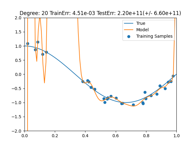
テスト誤差が最も小さいもの = 次数が3

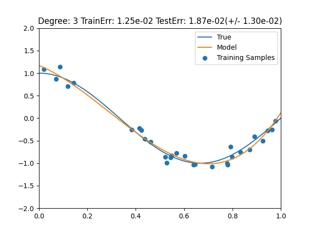
ここから如何に過学習がだめかということがわかる。

筑波大学の機械学習講座：課題のPythonスクリプト部分を作りながらsklearnを勉強する (3)

課題 3.2 多項式単回帰の訓練誤差とテスト誤差