まずはここで使う「単位円に内接/外接する多角形」と「その多角形の内接円/外接円」を描画するプログラムを掲示しておきます。三角関数を使っても複素数を使っても同じ結果となります。
正多角形の内接円と外接円(三角関数Ver.)

Regular_Polygon_draw01<-function(x) {
# グラフの色の決定
Black<-rgb(0,0,0)
Red<-rgb(1,0,0)
Magenta<-rgb(1,0,1)
Blue<-rgb(0,0,1)
Green<-rgb(0,1,0)
Cyan<-rgb(0,1,1)
Yellow<-rgb(1,1,0)
Gray<-"#888888"

# タイトル定義
Main_title<-c("Regular Polygon Draw(Physics method)")
x_title<-c("cos(x)")
y_title<-c("sin(x)")

# グラフのスケール決定
gs_x<-c(-1,1)
gs_y<-c(-1,1)
# y=sin(x)
f1_name<-c("Circumscribed circle")
c0<-seq(-pi,pi,length=100)
# y=2*sin(x)
f2_name<-c("Regular_Polygon")
c1<-seq(-pi,pi,length=x+1)
# y=3*sin(x)
f3_name<-c("Inscribed circle")
scl<-cos(pi/x)
# グラフ描画
plot(cos(c0),sin(c0),xlim=gs_x,ylim=gs_y,type="l",col=Black, main=Main_title,xlab=x_title,ylab=y_title)
par(new=T)#上書き指定
plot(cos(c1),sin(c1),xlim=gs_x,ylim=gs_y,type="l",col=Red, main="",xlab="",ylab="")
par(new=T)#上書き指定
plot(cos(c0)*scl,sin(c0)*scl,xlim=gs_x,ylim=gs_y,type="l",col=Black, main="",xlab="",ylab="")
# 基準線
abline(h=0)
abline(v=0)
# 凡例描画
legend("topleft", legend=c(f1_name,f2_name,f3_name),lty=c(1,1,1),col=c(Black,Red,Black))
}

library("animation")
Time_Code=c(3,3,4,4,5,5,6,6,7,7,8,8,9,9,10,11,12,13,14,15,20,25,30,35,40,45,50,60,70,80,90,100)
saveGIF({
for (i in Time_Code){
 Regular_Polygon_draw01(i)
}
}, interval = 0.1, movie.name = "TEST01.gif")
正多角形の内接円と外接円(複素数Ver.)

Regular_Polygon_draw02<-function(x) {
# グラフの色の決定
Black<-rgb(0,0,0)
Red<-rgb(1,0,0)
Magenta<-rgb(1,0,1)
Blue<-rgb(0,0,1)
Green<-rgb(0,1,0)
Cyan<-rgb(0,1,1)
Yellow<-rgb(1,1,0)
Gray<-"#888888"

# タイトル定義
Main_title<-c("Regular Polygon Draw(
Mathematical method)")
x_title<-c("Real number")
y_title<-c("Imaginary number")

# グラフのスケール決定
gs_x<-c(-1,1)
gs_y<-c(-1,1)
# Circumscribed circle(外接円)
f1_name<-c("Circumscribed circle")
f0<-function(x){exp(x*(0+1i))}
c1<-seq(-pi,pi,length=100)
c1_r<-Re(f0(c1))
c1_i<-Im(f0(c1))
# Regular_Polygon(正多角形)
f2_name<-c("Regular_Polygon")
c2<-seq(-pi,pi,length=x+1)
c2_r<-Re(f0(c2))
c2_i<-Im(f0(c2))

# Inscribed circle(内接円)
f3_name<-c("Inscribed circle")
scl<-cos(pi/x)
# グラフ描画
plot(c1_r,c1_i,xlim=gs_x,ylim=gs_y,type="l",col=Black, main=Main_title,xlab=x_title,ylab=y_title)
par(new=T)#上書き指定
plot(c2_r,c2_i,xlim=gs_x,ylim=gs_y,type="l",col=Red, main="",xlab="",ylab="")
par(new=T)#上書き指定
plot(c1_r*scl,c1_i*scl,xlim=gs_x,ylim=gs_y,type="l",col=Black, main="",xlab="",ylab="")
# 基準線
abline(h=0)
abline(v=0)
# 凡例描画
legend("topleft", legend=c(f1_name,f2_name,f3_name),lty=c(1,1,1),col=c(Black,Red,Black))
}

library("animation")
Time_Code=c(3,3,4,4,5,5,6,6,7,7,8,8,9,9,10,11,12,13,14,15,20,25,30,35,40,45,50,60,70,80,90,100)
saveGIF({
for (i in Time_Code){
 Regular_Polygon_draw02(i)
}
}, interval = 0.1, movie.name = "TEST01.gif")
単位円の内接多角形と外接多角形(複素数Verのみ)

Regular_Polygon_draw03<-function(x) {
# グラフの色の決定
Black<-rgb(0,0,0)
Red<-rgb(1,0,0)
Magenta<-rgb(1,0,1)
Blue<-rgb(0,0,1)
Green<-rgb(0,1,0)
Cyan<-rgb(0,1,1)
Yellow<-rgb(1,1,0)
Gray<-"#888888"

# タイトル定義
Main_title<-c("The Limit of inscribed polygons and circumscribed polygons")
x_title<-c("Real number")
y_title<-c("Imaginary number")

# グラフのスケール決定
gs_x<-c(-1,1)
gs_y<-c(-1,1)
# Circumscribed circle(外接多角形)
f1_name<-c("Circumscribed Polygon")
f0<-function(x){exp(x*(0+1i))}
c1<-seq(-pi,pi,length=x+1)
c1_r<-Re(f0(c1))
c1_i<-Im(f0(c1))
# Regular_Polygon(中間円)
f2_name<-c("Inner circle")
c2<-seq(-pi,pi,length=100)
c2_r<-Re(f0(c2))
c2_i<-Im(f0(c2))

# Inscribed circle(内接多角形)
f3_name<-c("Inscribed Polygon")
scl<-cos(pi/x)
# グラフ描画
plot(c1_r,c1_i,xlim=gs_x,ylim=gs_y,type="l",col=Green, main=Main_title,xlab=x_title,ylab=y_title)
par(new=T)#上書き指定
plot(c2_r*scl,c2_i*scl,xlim=gs_x,ylim=gs_y,type="l",col=Black, main="",xlab="",ylab="")
par(new=T)#上書き指定
plot(c1_r*scl,c1_i*scl,xlim=gs_x,ylim=gs_y,type="l",col=Blue, main="",xlab="",ylab="")
# 基準線
abline(h=0)
abline(v=0)
# 凡例描画
legend("topleft", legend=c(f1_name,f2_name,f3_name),lty=c(1,1,1),col=c(Green,Black,Blue))
}

library("animation")
Time_Code=c(3,3,4,4,5,5,6,6,7,7,8,8,9,9,10,11,12,13,14,15,20,25,30,35,40,45,50,60,70,80,90,100)
saveGIF({
for (i in Time_Code){
 Regular_Polygon_draw03(i)
}
}, interval = 0.1, movie.name = "TEST01.gif")
正方形(Square)/立方体(Cube)における内接円/球面の半径と外接円/球面の半径の連続推移
そもそも円描画関数r=sqrt(x^2+y^2+z^2…)(ただしrは半径,x,y,zは単位円/球面上の各座標軸におけるその値)の大源流は二項展開の例外(x+y)^2=x^2+y^2に遡るのです。
【初心者向け】パスカルの三角形と二項定理または二項展開
通常の二項展開(Binomial Expansion)の結果は
(x+y)^2=x^2+y^2+2xy
(x-y)^2=x^2+y^2-2xy
となる。
【初心者向け】ピタゴラスの定理あるいは三平方の定理からの出発
x=cos(θ),y=sin(θ)と置いた場合、余弦定理(Cosine Formula)から「θ=π/2ラジアン(90度)の時、cos(θ)^2=sin(θ)^2」が求められる。
# 余弦定理(Cosine Formula)で角度が90度の場合
a^2=(b-c)^2=b^2+c^2−2bc*cos(α)
# ところでα=90度(π/2ラジアン)の場合、cos(α)=0
a^2=b^2+c^2−2bc*0=b^2+c^2
虚数単位(Imaginary Unit)i^2=-1の概念を導入すると共益複素数(Conjugate Complex Number)r(0+1i)とr(0-1i)の打ち消し作用によってcos(θ)^2+sin(θ)^2が求められる。
# オイラーの公式(Euler's Formula)あるいは
# 共益複素数(Conjugate Complex Number)同士の打ち消し作用を用いた証明。
1=e^0=e^(iθ-iθ)=e^iθ-e^iθ)
=(cos(θ)+sin(θ)i)(cos(θ)-sin(θ)i)
=cos(θ)^2+sin(θ)i-sin(θ)i-sin(θ)i^2
=cos(θ)^2+sin(θ)^2 #i^2=-1
この時cos(θ)+sin(θ)は正方形の内接円/外接円の関係に従って「連続同心円」を描きます。

Square_XY<-function(Radius){
c0<-seq(-1,1,length=31)
cx<-c(rev(c0),c0[2:31])
c1<-seq(0,1,length=16)
cy<-c(c1,rev(c1[1:15]),-c1[2:16],-rev(c1[1:15]))
complex(real=cx*Radius,imaginary=cy*Radius)
}

c0<-seq(0,pi*2,length=61)
cx<-cos(c0)
cy<-sin(c0)
cmpx<-Re(Square_XY(1))
cmpy<-Im(Square_XY(1))

# 立方体における内接円/外接円の同心円的連鎖(周期1/2)描画
plot(cx,cy,type="l",xlim=c(-1,1),asp=1,ylim=c(-1,1),main="Square
& Inscribed/Circumscribed Circle",xlab="",ylab="", col=rgb(0,1,0))
par(new=T)
plot(cx*sqrt(2)/2,cy*sqrt(2)/2,type="l",xlim=c(-1,1),asp=1,ylim=c(-1,1),main="",xlab="",ylab="",col=rgb(0,1,0))
par(new=T)
plot(cx*2/sqrt(2),cy*2/sqrt(2),type="l",xlim=c(-1,1),asp=1,ylim=c(-1,1),main="",xlab="",ylab="",col=c(200,200,200))
par(new=T)
plot(cx/2,cy/2,type="l",xlim=c(-1,1),asp=1,ylim=c(-1,1),main="",xlab="",ylab="", col=c(200,200,200))
par(new=T)
plot(cx*2,cy*2,type="l",xlim=c(-1,1),asp=1,ylim=c(-1,1),main="",xlab="",ylab="", col=c(200,200,200))

# 正方形
par(new=T)
plot(cmpx,cmpy,type="l",xlim=c(-1,1),asp=1,ylim=c(-1,1),main="",xlab="",ylab="",col=rgb(1,0,0))
par(new=T)
plot(cmpx*sqrt(2)/2,cmpy*sqrt(2)/2,type="l",xlim=c(-1,1),asp=1,ylim=c(-1,1),main="",xlab="",ylab="",col=c(200,200,200))
par(new=T)
plot(cmpx*2/sqrt(2),cmpy*2/sqrt(2),type="l",xlim=c(-1,1),asp=1,ylim=c(-1,1),main="",xlab="",ylab="",col=c(200,200,200))
par(new=T)
plot(cmpx/2,cmpy/2,type="l",xlim=c(-1,1),asp=1,ylim=c(-1,1),main="",xlab="",ylab="", col=c(200,200,200))
par(new=T)
plot(cmpx*2,cmpy*2,type="l",xlim=c(-1,1),asp=1,ylim=c(-1,1),main="",xlab="",ylab="", col=c(200,200,200))

abline(h=0,col=rgb(0,0,0))
abline(v=0,col=rgb(0,0,0))
単位円筒(Unit Cylinder)との関係
【初心者向け】物理学における「単位円筒(Unit Cylinder)」の概念について。
【初心者向け】「単位円筒」から「単位球面」へ


# 正方形
library(rgl)
Rtime<-seq(0,2,length=5)
tr01<-c(1,(0+1i),-1,(0-1i),1)
Real<-Re(tr01)
Imag<-Im(tr01)
plot3d(Real,Imag,Rtime,type="l",xlim=c(-1,1),ylim=c(-1,1),zlim=c(0,2))
movie3d(spin3d(axis=c(0,0,1),rpm=5),duration=10,fps=25,movie="~/Desktop/test16")
単位円(Unit circle)上に同心円を描く任意の正方形内で正方形を回すと、その辺長の比はsqrt(2):sqrt(2)と1:2の間を反復し続けますが、この比が多層化された内接円と外接円の半径の推移比とぴったり重なるのです。
【初心者向け】ピタゴラスの定理あるいは三平方の定理からの出発

【Rで球面幾何学】式Cos(θ)+Sin(θ)(i)から式Cos(θ)+Cos(θ-π/NoS)(i)(NoS=Number of Sides)への「自然な」拡張について。
| Target_size | Target_names | Target_values | |
|---|---|---|---|
| 1 | 2^-1 | 2^-1(2^-0.5r) | 0.5 |
| 2 | 2^-1 | 2^-1d=2^-1*4 | 1 |
| 3 | 2^-1 | 2^-1a1=2^0a0 | sqrt(2)=1.414214 |
| 4 | 2^-1 | 2^-1a1(2^-0.5a0)*4 | 4sqrt(2)=5.656854 |
| 5 | 2^-0.5 | 2^-0.5(2^0r) | sqrt(2)/2=0.7071068 |
| 6 | 2^-0.5 | 2^-0.5d=2^-0.5*4 | sqrt(2)=1.414214 |
| 7 | 2^-0.5 | 2^-0.5a1=2^0a0 | 1 |
| 8 | 2^-0.5 | 2^-1a1(2^0.5a0)*4 | 4 |
| 9 | 2^0 | 2^0(2^-0.5R,2^0.5r) | 1 |
| 10 | 2^0 | 2^0d=2^0*4 | 2 |
| 11 | 2^0 | 2^0a1=2^0.5a0 | sqrt(8)=2sqrt(2)=2.828427 |
| 12 | 2^0 | 2^0a1(2^0.5a0)*4 | sqrt(32)=4sqrt(2)=5.656854 |
| 13 | 2^0.5 | 2^0.5(2^-0R,2^1r) | sqrt(2)=1.414214 |
| 14 | 2^0.5 | 2^0.5d=2^0.5*4 | 2sqrt(2)=2.828427 |
| 15 | 2^0.5 | 2^0.5a1=2^1a0 | 4 |
| 16 | 2^0.5 | 2^0.5a1(2^0a0)*4 | 8 |
| 17 | 2^1 | 2^1(2^1-0.5R,2^0.5r) | 2 |


この規則正しさはコサイン波もサイン波も「四分割した上で90度ずつ位相をずらして再構成しても同じ波形になる」特徴に由来しています。
【Rで球面幾何学】何故「正方形」ではCos(θ)+Sin(θ)iが成立するのか?

ところで立方体(正六面体)に内接/外接する同心球面の半径の推移は以下となり、双対関係にある正八面体のそれと一致するのです。
正多面体の計量と真球率
# r1=1辺aの立方体(正六面体)に内接する球面の半径
> a<-1
> a/2
[1] 0.5

# R1=1辺aの立方体(正六面体)に外接する球面の半径
> a<-1
> a*sqrt(3)/2
[1] 0.8660254

# 立方体(正六面体)の真球率(r/R)
> 0.5/0.8660254
[1] 0.5773503
> sqrt(3)/3
[1] 0.5773503

# r2=1辺aの正八面体に内接する球面の半径
> a<-1
> a*sqrt(6)/6
[1] 0.4082483

# R2=1辺aの正八面体に外接する球面の半径
> a<-1
> a*sqrt(2)/2
[1] 0.7071068

# 立方体(正六面体)の真球率(r/R)
> 0.4082483/0.7071068
[1] 0.5773503
> sqrt(3)/3
[1] 0.5773503

# 真球率が一致するという事はこの二つの図形が双対関係にある事を意味する
どうやらこれが2^n3^m集に含まれる多面体の構築する同心球面の特徴と言えそうです。
【オイラーの多面体定理と正多面体】とある「球面幾何学(Spherical Geometry)」の出発点…
正三角形(Equilateral Triangle)/正四面体(Regular Tetrahedron)/正六角形(Regular Hexagon)における内接円/球面の半径と外接円/球面の半径の連続推移
「連続同心円を構築する」性質そのものは正三角形も備えています。

単位円筒(Unit Cylinder)との関係
【初心者向け】物理学における「単位円筒(Unit Cylinder)」の概念について。
【初心者向け】「単位円筒」から「単位球面」へ


# 正三角形
library(rgl)
Rtime<-seq(0,2,length=4)
tr01<-c(1,(-1+sqrt(3)*(0+1i))/2,(-1-sqrt(3)*(0+1i))/2,1)
Real<-Re(tr01)
Imag<-Im(tr01)
# plot(Real,Imag,type="l")
plot3d(Real,Imag,Rtime,type="l",xlim=c(-1,1),ylim=c(-1,1),zlim=c(0,2))
movie3d(spin3d(axis=c(0,0,1),rpm=5),duration=10,fps=25,movie="~/Desktop/test11")
| Target_size | Target_names | Target_values | |
|---|---|---|---|
| 1 | 3^-1 | 3^-1(3^0r) | 1/2=0.5 |
| 2 | 3^-1 | 3^-1h=3^-1*3 | 3/2=1.5 |
| 3 | 3^-1 | 3^-1a1=3^0a0 | 2*sqrt(1.5)=2.44949 |
| 4 | 3^-1 | 3^-1a1(3^0a0)*3 | 6*sqrt(1.5)=7.348469 |
| 5 | 3^0 | 3^0(3^-1R,3^1r) | 1.0 |
| 6 | 3^0 | 3^0h=3^0*3 | 3.0 |
| 7 | 3^0 | 3^0a1=3^1a0 | 2*sqrt(3)=3.464102 |
| 8 | 3^0 | 3^0a1(3^1a0)*3 | 6*sqrt(3)=10.3923 |
| 9 | 3^1 | 3^1(3^0R) | 3.0 |
target_size<-c("3^-1","3^-1","3^-1","3^-1","3^0","3^0","3^0","3^0","3^1")

target_names<-c("3^-1(3^0r)","3^-1h=3^-1*3","3^-1a1=3^0a0","3^-1a1(3^0a0)*3","3^0(3^-1R,3^1r)","3^0h=3^0*3","3^0a1=3^1a0","3^0a1(3^1a0)*3","3^1(3^0R)")

target_values<-c("1/2=0.5","3/2=1.5","2*sqrt(1.5)=2.44949","6*sqrt(1.5)=7.348469","1.0","3.0","2*sqrt(3)=3.464102","6*sqrt(3)=10.3923","3.0")

Regula_falsi03<-data.frame(Target_size=target_size,Target_names=target_names,Target_values=target_values)
library(xtable)
print(xtable(Regula_falsi03), type = "html")
単位円(Unit circle)上に同心円を描く任意の正三角形内で正三角形を回すと、その辺長の比は2:2と1:2の間を反復し続けますが、この比が多層化された内接円と外接円の半径の推移比とぴったり重なるのです。

Three_square_theorem03<-function(x){
c0<-c(0,2/3*pi,-2/3*pi,0)
c0_cos<-cos(c0)
c0_sin<-sin(c0)
plot(c0_cos,c0_sin,type="l",xlim=c(-1,1),ylim=c(-1,1),main="Regular polygon rotation",xlab="Cos(θ)",ylab="Sin(θ)")
text(c0_cos,c0_sin, labels=c("a","b","c",""),col=c(rgb(1,0,0),rgb(1,0,0),rgb(1,0,0),rgb(1,0,0)),cex=c(2,2,2,2))
line_scale_01_cos<-seq(cos(c0[1]),cos(c0[2]),length=15)
line_scale_01_sin<-seq(sin(c0[1]),sin(c0[2]),length=15)
line_scale_02_cos<-seq(cos(c0[2]),cos(c0[3]),length=15)
line_scale_02_sin<-seq(sin(c0[2]),sin(c0[3]),length=15)
line_scale_03_cos<-seq(cos(c0[3]),cos(c0[1]),length=15)
line_scale_03_sin<-seq(sin(c0[3]),sin(c0[1]),length=15)
text(c(line_scale_01_cos[x],line_scale_02_cos[x],line_scale_03_cos[x]),c(line_scale_01_sin[x],line_scale_02_sin[x],line_scale_03_sin[x]), labels=c("ab","bc","ca"),col=c(rgb(0,0,1),rgb(0,0,1),rgb(0,0,1)),cex=c(2,2,2))

# 塗りつぶし
polygon(c(c0_cos[1],line_scale_03_cos[x],line_scale_01_cos[x],c0_cos[1]), #x
c(c0_sin[1],line_scale_03_sin[x],line_scale_01_sin[x],c0_sin[1]), #y
density=c(30), #塗りつぶす濃度
angle=c(45),     #塗りつぶす斜線の角度
col=rgb(0,1,0))

# 塗りつぶし
polygon(c(c0_cos[2],line_scale_01_cos[x],line_scale_02_cos[x],c0_cos[2]), #x
c(c0_sin[2],line_scale_01_sin[x],line_scale_02_sin[x],c0_sin[2]), #y
density=c(30), #塗りつぶす濃度
angle=c(45),     #塗りつぶす斜線の角度
col=rgb(0,1,0))

# 塗りつぶし
polygon(c(c0_cos[3],line_scale_02_cos[x],line_scale_03_cos[x],c0_cos[3]), #x
c(c0_sin[3],line_scale_02_sin[x],line_scale_03_sin[x],c0_sin[3]), #y
density=c(30), #塗りつぶす濃度
angle=c(45),     #塗りつぶす斜線の角度
col=rgb(0,1,0))

}

# アニメーション
library("animation")
Time_Code=c(1,2,3,4,5,6,7,8,9,10,11,12,13,14,15)
saveGIF({
for (i in Time_Code){
 Three_square_theorem03(i)
}
}, interval = 0.1, movie.name = "TEST003.gif")
【Rで球面幾何学】何故「正方形」ではCos(θ)+Sin(θ)iが成立するのか?

ただここから先はcos(θ)+sin(θ)(i)が成立せず、その一般形たるCos(θ)+Cos(θ-π/NoS)i(NoS=Number of Sides)で考えないといけなくなります。

c0=seq(0,2*pi,length=7)
c1=c(2,4,2,4,2,4,2)
c2=c(1,2,1,2,1,2,1)
c3=c(1/2,1,1/2,1,1/2,1,1/2)
plot(c0,c1,type="o",xlim=c(0,2*pi),ylim=c(1/2,4),ylab='x', xlab='y')
par(new=T) #上書き
plot(c0,c2,type="o",xlim=c(0,2*pi),ylim=c(1/2,4),ylab='', xlab='')
par(new=T) #上書き
plot(c0,c3,type="o",xlim=c(0,2*pi),ylim=c(1/2,4), main="Expected Multilayered Tori", ylab='', xlab='')
# 外接円=内接円による境界線
abline(h=2,col=rgb(1,0,0))
abline(h=1,col=rgb(0,1,0))
abline(h=0.5,col=rgb(0,0,1))
# 凡例
legend("bottomright", legend=c("Mj=2+Mn,Mn=1","Mj=1+Mn,Mn=1/2","Mj=1/2+Mn,Mn=1/4"), lty=c(1,1,1), col=c(rgb(1,0,0),rgb(0,1,0),rgb(0,0,1)))

R_time=seq(0,2*pi,length=300)
Smp_time=seq(0,2/3*pi,length=100)

# 標準円(半径0.5→1)
f0<-function(x){cos(x-1/3*pi)}
S_data<-c(f0(Smp_time),f0(Smp_time),f0(Smp_time))
plot(R_time,S_data,type="l",xlim=c(0,2*pi),ylim=c(0.5,4),main="Torus  drawn by circumscribed and inscribed circle",ylab='Circumference(radian)', xlab='Circle radius')
# 半径1→2
par(new=T) #上書き
S_data<-c(f0(Smp_time)*2,f0(Smp_time)*2,f0(Smp_time)*2)
plot(R_time,S_data,type="l",xlim=c(0,2*pi),ylim=c(0.5,4),ylab='', xlab='')

# 半径2→4)
par(new=T) #上書き
S_data<-c(f0(Smp_time)*4,f0(Smp_time)*4,f0(Smp_time)*4)
plot(R_time,S_data,type="l",xlim=c(0,2*pi),ylim=c(0.5,4),ylab='', xlab='')
# 外接円=内接円による境界線
abline(h=2,col=rgb(1,0,0))
abline(h=1,col=rgb(0,1,0))
abline(h=0.5,col=rgb(0,0,1))
# 凡例
legend("bottomright", legend=c("Mj=2+Mn,Mn=1","Mj=1+Mn,Mn=1/2","Mj=1/2+Mn,Mn=1/4"), lty=c(1,1,1), col=c(rgb(1,0,0),rgb(0,1,0),rgb(0,0,1)))
ところで正三角形(Equilateral Triangle)を最小の操作で立体に拡張した正四面体(Regular Tetrahedron)に内接/外接する同心球面の半径の推移は以下となります。
正多面体の計量と真球率
# r=1辺aの正四面体に内接する球面の半径
> a<-1
> a*sqrt(6)/12
[1] 0.2041241

# R1=1辺aの正四面体に外接する球面の半径
> a<-1
> a*sqrt(6)/4
[1] 0.6123724

# 正四面体の真球率(r/R)
> 0.2041241/0.6123724
[1] 0.3333333
> 1/3
[1] 0.3333333
ただし単体で平面充填性を備える正三角形と異なり、正四面体は単体では立体充填性を備えておらず、その性質を備えるには正八面体と交互に組み合わせないといけません。
【オイラーの多面体定理と正多面体】正四面体と正六面体と正八面体の連続性と「テトラパックの思わぬ正体」について。
単体で平面充填性を備える正方形や単体で立体充填性を備える立方体の場合はその自己相似形再現サイクルが平方数(Square Number)(0,1,4,9,16,25,36,49,64,81,100…)や立方数(Cubic Number)(0,1,8,27,64,125…)に従う為に「(面を中心とする)偶数系展開」と「(頂点を中心とする)奇数系展開」が交互に現れます。
正方形による平面充填(面を基点とした場合)…コサイン波の振る舞いに対応。
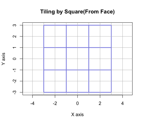
# Tiling(Plane Filling) by Square(From Face)
cx=c(-3,3,3,-3,-3)
cy=c(-3,-3,3,3,-3)
plot(cx,cy,type="l",asp=1,xlim=c(-3,3),ylim=c(-3,3),col=rgb(0,0,1),lwd=2, main="Tiling by Square(From Face)",xlab="X axis",ylab="Y axis")

lines(c(-3,3), c(-1,-1),col=rgb(0,0,1),lwd=2)
lines(c(-3,3), c(1,1),col=rgb(0,0,1),lwd=2)
lines(c(-1,-1), c(-3,3),col=rgb(0,0,1),lwd=2)
lines(c(1,1), c(-3,3),col=rgb(0,0,1),lwd=2)

# 方眼(Square Grid)
for (i in -5:5) {
abline(h = i,col=c(200,200,200))
abline(v = i,col=c(200,200,200))
 }
正方形による平面充填(頂点を基点とした場合)…サイン波の振る舞いに対応。
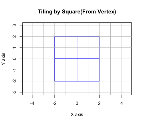
# Tiling(Plane Filling) by Square(From Vertex)
cx=c(-2,2,2,-2,-2)
cy=c(-2,-2,2,2,-2)
plot(cx,cy,type="l",asp=1,xlim=c(-3,3),ylim=c(-3,3),col=rgb(0,0,1),lwd=2, main="Tiling by Square(From Vertex)",xlab="X axis",ylab="Y axis")

lines(c(-2,2), c(0,0),col=rgb(0,0,1),lwd=2)
lines(c(0,0), c(-2,2),col=rgb(0,0,1),lwd=2)

# 方眼(Square Grid)
for (i in -5:5) {
abline(h = i,col=c(200,200,200))
abline(v = i,col=c(200,200,200))
 }
虚数単位(Imaginary Unit)i^2=-1導入により複素数cos(θ)+sin(θ)iが複素平面上に円を描くのは基本的にこの性質に立脚しているのです。
【Rで球面幾何学】そもそも複素数Xi(x*(0+1i))はどう振る舞う?


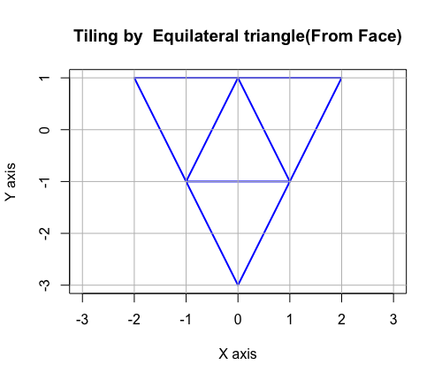
ところが正三角形の自己相似形再現サイクルの場合、そもそも「偶数系」と「奇数系」が交互に現れません。
正三角形による平面充填(面を基点とした場合)
# Tiling(Plane Filling) by Equilateral triangle(From Face)
cx=c(-2,2,0,-2)
cy=c(1,1,-3,1)
plot(cx,cy,type="l",asp=1,xlim=c(-2,2),ylim=c(-3,1),col=rgb(0,0,1),lwd=2, main="Tiling by  Equilateral triangle(From Face)",xlab="X axis",ylab="Y axis")

lines(c(-1,0), c(-1,1),col=rgb(0,0,1),lwd=2)
lines(c(0,1), c(1,-1),col=rgb(0,0,1),lwd=2)
lines(c(-1,1), c(-1,-1),col=rgb(0,0,1),lwd=2)

# 方眼(Square Grid)
for (i in -5:5) {
abline(h = i,col=c(200,200,200))
abline(v = i,col=c(200,200,200))
 }
正三角形による平面充填(頂点を基点とした場合)
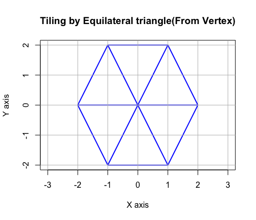
# Tiling(Plane Filling) by Equilateral triangle(From Vertex)
cx=c(-2,-1,1,2,1,-1,-2)
cy=c(0,2,2,0,-2,-2,0)
plot(cx,cy,type="l",asp=1,xlim=c(-2,2),ylim=c(-2,2),col=rgb(0,0,1),lwd=2, main="Tiling by Equilateral triangle(From Vertex)",xlab="X axis",ylab="Y axis")

lines(c(-1,1), c(-2,2),col=rgb(0,0,1),lwd=2)
lines(c(-1,1), c(2,-2),col=rgb(0,0,1),lwd=2)
lines(c(-2,2), c(0,0),col=rgb(0,0,1),lwd=2)

# 方眼(Square Grid)
for (i in -5:5) {
abline(h = i,col=c(200,200,200))
abline(v = i,col=c(200,200,200))
 }
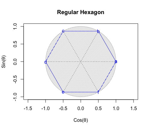
ちなみに正三角形は正六角形と「頂点と面を交換する双対変換操作によって互いに変換される双対関係」にあり、どちらも平面充当性を備えていますが、もはや連続同心円は構築しません。

単位円筒(Unit Cylinder)との関係
【初心者向け】物理学における「単位円筒(Unit Cylinder)」の概念について。
【初心者向け】「単位円筒」から「単位球面」へ


統計言語Rによる作図例
# 正6角形
library(rgl)
Rtime<-seq(0,2,length=7)
tr01<-c(1,(1+sqrt(3)*(0+1i))/2,(-1+sqrt(3)*(0+1i))/2,-1,(-1-sqrt(3)*(0+1i))/2,(1-sqrt(3)*(0+1i))/2,1)
Real<-Re(tr01)
Imag<-Im(tr01)
# plot(Real,Imag,type="l")
plot3d(Real,Imag,Rtime,type="l",xlim=c(-1,1),ylim=c(-1,1),zlim=c(0,2))
movie3d(spin3d(axis=c(0,0,1),rpm=5),duration=10,fps=25,movie="~/Desktop/test13")

Three_square_theorem06<-function(x){
c0<-seq(0,2*pi,length=7)
c0_cos<-cos(c0)
c0_sin<-sin(c0)
plot(c0_cos,c0_sin,type="l",main="Regular polygon rotation",xlab="Cos(θ)",ylab="Sin(θ)")
text(c0_cos,c0_sin, labels=c("a","b","c","d","e","f",""),col=c(rgb(1,0,0),rgb(1,0,0),rgb(1,0,0),rgb(1,0,0),rgb(1,0,0),rgb(1,0,0),rgb(1,0,0)),cex=c(2,2,2,2,2,2,2))
line_scale_01_cos<-seq(cos(c0[1]),cos(c0[2]),length=15)
line_scale_01_sin<-seq(sin(c0[1]),sin(c0[2]),length=15)
line_scale_02_cos<-seq(cos(c0[2]),cos(c0[3]),length=15)
line_scale_02_sin<-seq(sin(c0[2]),sin(c0[3]),length=15)
line_scale_03_cos<-seq(cos(c0[3]),cos(c0[4]),length=15)
line_scale_03_sin<-seq(sin(c0[3]),sin(c0[4]),length=15)
line_scale_04_cos<-seq(cos(c0[4]),cos(c0[5]),length=15)
line_scale_04_sin<-seq(sin(c0[4]),sin(c0[5]),length=15)
line_scale_05_cos<-seq(cos(c0[5]),cos(c0[6]),length=15)
line_scale_05_sin<-seq(sin(c0[5]),sin(c0[6]),length=15)
line_scale_06_cos<-seq(cos(c0[6]),cos(c0[1]),length=15)
line_scale_06_sin<-seq(sin(c0[6]),sin(c0[1]),length=15)
text(c(line_scale_01_cos[x],line_scale_02_cos[x],line_scale_03_cos[x],line_scale_04_cos[x],line_scale_05_cos[x],line_scale_06_cos[x]),c(line_scale_01_sin[x],line_scale_02_sin[x],line_scale_03_sin[x],line_scale_04_sin[x],line_scale_05_sin[x],line_scale_06_sin[x]), labels=c("ab","bc","cd","de","ef","fa",""),col=c(rgb(0,0,1),rgb(0,0,1),rgb(0,0,1),rgb(0,0,1),rgb(0,0,1),rgb(0,0,1),rgb(0,0,1)),cex=c(2,2,2,2,2,2,2))

# 塗りつぶし
polygon(c(c0_cos[1],line_scale_06_cos[x],line_scale_01_cos[x],c0_cos[1]), #x
c(c0_sin[1],line_scale_06_sin[x],line_scale_01_sin[x],c0_sin[1]), #y
density=c(30), #塗りつぶす濃度
angle=c(45),     #塗りつぶす斜線の角度
col=rgb(0,1,0))

# 塗りつぶし
polygon(c(c0_cos[2],line_scale_01_cos[x],line_scale_02_cos[x],c0_cos[2]), #x
c(c0_sin[2],line_scale_01_sin[x],line_scale_02_sin[x],c0_sin[2]), #y
density=c(30), #塗りつぶす濃度
angle=c(45),     #塗りつぶす斜線の角度
col=rgb(0,1,0))

# 塗りつぶし
polygon(c(c0_cos[3],line_scale_02_cos[x],line_scale_03_cos[x],c0_cos[3]), #x
c(c0_sin[3],line_scale_02_sin[x],line_scale_03_sin[x],c0_sin[3]), #y
density=c(30), #塗りつぶす濃度
angle=c(45),     #塗りつぶす斜線の角度
col=rgb(0,1,0))

# 塗りつぶし
polygon(c(c0_cos[4],line_scale_03_cos[x],line_scale_04_cos[x],c0_cos[4]), #x
c(c0_sin[4],line_scale_03_sin[x],line_scale_04_sin[x],c0_sin[4]), #y
density=c(30), #塗りつぶす濃度
angle=c(45),     #塗りつぶす斜線の角度
col=rgb(0,1,0))

# 塗りつぶし
polygon(c(c0_cos[5],line_scale_04_cos[x],line_scale_05_cos[x],c0_cos[5]), #x
c(c0_sin[5],line_scale_04_sin[x],line_scale_05_sin[x],c0_sin[5]), #y
density=c(30), #塗りつぶす濃度
angle=c(45),     #塗りつぶす斜線の角度
col=rgb(0,1,0))
# 塗りつぶし
polygon(c(c0_cos[6],line_scale_05_cos[x],line_scale_06_cos[x],c0_cos[6]), #x
c(c0_sin[6],line_scale_05_sin[x],line_scale_06_sin[x],c0_sin[6]), #y
density=c(30), #塗りつぶす濃度
angle=c(45),     #塗りつぶす斜線の角度
col=rgb(0,1,0))

}

# アニメーション
library("animation")
Time_Code=c(1,2,3,4,5,6,7,8,9,10,11,12,13,14,15)
saveGIF({
for (i in Time_Code){
 Three_square_theorem06(i)
}
}, interval = 0.1, movie.name = "TEST06.gif")
| Target_size | Target_names | Target_values | |
|---|---|---|---|
| 1 | 6^-1 | 6^-1 | 1/6=0.1666666 |
| 2 | 6^-1 | 6^-1a1 | 1/6*1.154701=0.1924502 |
| 3 | 6^-1 | 6^-1a1*6 | 0.1924502*6=1.154701 |
| 4 | 6^-0.8394411 | 6^-0.8394411 | 0.1924502*1.154701=0.2222224 |
| 5 | ... | ... | ... |
| 6 | 6^-0.08027941 | 6^-0.08027921 | -0.8660254 |
| 7 | 6^0 | 6^0a0 | 1.0 |
| 8 | 6^0 | 6^0a0*6 | 6.0 |
| 9 | 6^0 | 6^0 | 1.0 |
| 10 | 6^0 | 6^0a1 | 1.333333 |
| 11 | 6^0 | 6^0a1*6 | 1.333333*6=7.999998 |
| 12 | 6^0.08027895 | 6^0.08027895 | 1.333333*0.8660254=1.333334 |
| 13 | ... | ... | ... |
| 14 | 6^0.7591625 | 6^0.7591625 | 4.500001*0.8660254=3.897115 |
| 15 | 6^1 | 6^1a0 | 6/1.333333=4.500001 |
| 16 | 6^1 | 6^1a0*6 | 4.500001*6=27.00001 |
| 17 | 6^1 | 6^1 | 6.0 |
target_size<-c("6^-1","6^-1","6^-1","6^-0.8394411","...","6^-0.08027941","6^0","6^0","6^0","6^0","6^0","6^0.08027895","...","6^0.7591625","6^1","6^1","6^1")

target_names<-c("6^-1","6^-1a1","6^-1a1*6","6^-0.8394411","...","6^-0.08027921","6^0a0","6^0a0*6","6^0","6^0a1","6^0a1*6","6^0.08027895","...","6^0.7591625","6^1a0","6^1a0*6","6^1")

target_values<-c("1/6=0.1666666","1/6*1.154701=0.1924502","0.1924502*6=1.154701","0.1924502*1.154701=0.2222224","...","-0.8660254","1.0","6.0","1.0","1.333333","1.333333*6=7.999998","1.333333*0.8660254=1.333334","...","4.500001*0.8660254=3.897115","6/1.333333=4.500001","4.500001*6=27.00001","6.0")

Regula_falsi06<-data.frame(Target_size=target_size,Target_names=target_names,Target_values=target_values)
library(xtable)
print(xtable(Regula_falsi06), type = "html")
【Rで球面幾何学】何故「正方形」ではCos(θ)+Sin(θ)iが成立するのか?

どうやらこれが3^m集に含まれる多面体の構築する同心球面の特徴と言えそうです。そして正四面体から立方体(正六面体)や正八面体への変換操作は3^m集の構築する同心球面空間から2^n3^mの構築する同心球面空間への乗り換えという話になってきそうです。
【オイラーの多面体定理と正多面体】とある「球面幾何学(Spherical Geometry)」の出発点…
正五角形(Pentagon)/正十二面体(Regular Dodecahedron)/正二十面体(Regular Icosahedron)における内接円/球面の半径と外接円/球面の半径の推移
正三角形や正方形と異なり、正五角形以上の正多角形の外接/内接円はもはや連続同心円を構築しません。

単位円筒(Unit Cylinder)との関係
【初心者向け】物理学における「単位円筒(Unit Cylinder)」の概念について。
【初心者向け】「単位円筒」から「単位球面」へ


# 正5角形
library(rgl)
Rtime<-seq(0,2,length=6)
tr01<-c(1,(-1+sqrt(5)+(0+1i)*sqrt(10+2*sqrt(5)))/4,(-1-sqrt(5)+(0+1i)*sqrt(10-2*sqrt(5)))/4,(-1-sqrt(5)-(0+1i)*sqrt(10-2*sqrt(5)))/4,(-1+sqrt(5)-(0+1i)*sqrt(10+2*sqrt(5)))/4,1)
Real<-Re(tr01)
Imag<-Im(tr01)
# plot(Real,Imag,type="l")
plot3d(Real,Imag,Rtime,type="l",xlim=c(-1,1),ylim=c(-1,1),zlim=c(0,2))
movie3d(spin3d(axis=c(0,0,1),rpm=5),duration=10,fps=25,movie="~/Desktop/test13")

Three_square_theorem05<-function(x){
c0<-seq(0,2*pi,length=6)
c0_cos<-cos(c0)
c0_sin<-sin(c0)
plot(c0_cos,c0_sin,type="l",main="Regular polygon rotation",xlab="Cos(θ)",ylab="Sin(θ)")
text(c0_cos,c0_sin, labels=c("a","b","c","d","e",""),col=c(rgb(1,0,0),rgb(1,0,0),rgb(1,0,0),rgb(1,0,0),rgb(1,0,0),rgb(1,0,0)),cex=c(2,2,2,2,2,2))
line_scale_01_cos<-seq(cos(c0[1]),cos(c0[2]),length=15)
line_scale_01_sin<-seq(sin(c0[1]),sin(c0[2]),length=15)
line_scale_02_cos<-seq(cos(c0[2]),cos(c0[3]),length=15)
line_scale_02_sin<-seq(sin(c0[2]),sin(c0[3]),length=15)
line_scale_03_cos<-seq(cos(c0[3]),cos(c0[4]),length=15)
line_scale_03_sin<-seq(sin(c0[3]),sin(c0[4]),length=15)
line_scale_04_cos<-seq(cos(c0[4]),cos(c0[5]),length=15)
line_scale_04_sin<-seq(sin(c0[4]),sin(c0[5]),length=15)
line_scale_05_cos<-seq(cos(c0[5]),cos(c0[1]),length=15)
line_scale_05_sin<-seq(sin(c0[5]),sin(c0[1]),length=15)
text(c(line_scale_01_cos[x],line_scale_02_cos[x],line_scale_03_cos[x],line_scale_04_cos[x],line_scale_05_cos[x]),c(line_scale_01_sin[x],line_scale_02_sin[x],line_scale_03_sin[x],line_scale_04_sin[x],line_scale_05_sin[x]), labels=c("ab","bc","cd","de","ea",""),col=c(rgb(0,0,1),rgb(0,0,1),rgb(0,0,1),rgb(0,0,1),rgb(0,0,1),rgb(0,0,1)),cex=c(2,2,2,2,2,2))

# 塗りつぶし
polygon(c(c0_cos[1],line_scale_05_cos[x],line_scale_01_cos[x],c0_cos[1]), #x
c(c0_sin[1],line_scale_05_sin[x],line_scale_01_sin[x],c0_sin[1]), #y
density=c(30), #塗りつぶす濃度
angle=c(45),     #塗りつぶす斜線の角度
col=rgb(0,1,0))

# 塗りつぶし
polygon(c(c0_cos[2],line_scale_01_cos[x],line_scale_02_cos[x],c0_cos[2]), #x
c(c0_sin[2],line_scale_01_sin[x],line_scale_02_sin[x],c0_sin[2]), #y
density=c(30), #塗りつぶす濃度
angle=c(45),     #塗りつぶす斜線の角度
col=rgb(0,1,0))

# 塗りつぶし
polygon(c(c0_cos[3],line_scale_02_cos[x],line_scale_03_cos[x],c0_cos[3]), #x
c(c0_sin[3],line_scale_02_sin[x],line_scale_03_sin[x],c0_sin[3]), #y
density=c(30), #塗りつぶす濃度
angle=c(45),     #塗りつぶす斜線の角度
col=rgb(0,1,0))

# 塗りつぶし
polygon(c(c0_cos[4],line_scale_03_cos[x],line_scale_04_cos[x],c0_cos[4]), #x
c(c0_sin[4],line_scale_03_sin[x],line_scale_04_sin[x],c0_sin[4]), #y
density=c(30), #塗りつぶす濃度
angle=c(45),     #塗りつぶす斜線の角度
col=rgb(0,1,0))

# 塗りつぶし
polygon(c(c0_cos[5],line_scale_04_cos[x],line_scale_05_cos[x],c0_cos[5]), #x
c(c0_sin[5],line_scale_04_sin[x],line_scale_05_sin[x],c0_sin[5]), #y
density=c(30), #塗りつぶす濃度
angle=c(45),     #塗りつぶす斜線の角度
col=rgb(0,1,0))

}

# アニメーション
library("animation")
Time_Code=c(1,2,3,4,5,6,7,8,9,10,11,12,13,14,15)
saveGIF({
for (i in Time_Code){
 Three_square_theorem05(i)
}
}, interval = 0.1, movie.name = "TEST005.gif")
| Target_size | Target_names | Target_values | |
|---|---|---|---|
| 1 | 5^-1 | 5^-1 | 1/5=0.2 |
| 2 | 5^-1 | 5^-1d | (1+sqrt(5))/2*0.2=0.3236068 |
| 3 | 5^-1 | 5^-1a1 | 0.2*1.796112=0.3592224 |
| 4 | 5^-1 | 5^-1a1*5 | 0.3592224*5=1.796112 |
| 5 | 5^-0.2722623 | 5^-0.2722623 | 0.3592224*1.796112=-0.2722623 |
| 6 | ... | ... | ... |
| 7 | 5^-0.131683 | 5^-0.131683 | 0.8090168 |
| 8 | 5^0 | 5^0a0 | 1/1.453085=0.688191 |
| 9 | 5^0 | 5^0a0*5 | 0.5567581*5=3.440955 |
| 10 | 5^0 | 5^0=1 | 1.0 |
| 11 | 5^0 | 5^0d | (1+sqrt(5))/2=1.618034 |
| 12 | 5^0 | 5^0a1 | 1.796112 |
| 13 | 5^0 | 5^0a1*5 | 1.796112*5=8.98056 |
| 14 | 5^0.1316829 | 5^0.7277376 | 1.796112*1.796112=3.226018 |
| 15 | ... | ... | ... |
| 16 | 5^0.535628 | 5^0.535628 | 3.440955*1.453085=2.368034 |
| 17 | 5^1 | 5^0a1 | 5/1.453085=3.440955 |
| 18 | 5^1 | 5^0a1*5 | 3.440955*5=17.20478 |
| 19 | 5^1 | 5^1 | 5 |
| 20 | 5^1 | 5^1d | ((1+sqrt(5))/2)*5=8.09017 |
target_size<-c("5^-1","5^-1","5^-1","5^-1","5^-0.2722623","...","5^-0.131683","5^0","5^0","5^0","5^0","5^0","5^0","5^0.1316829","...","5^0.535628","5^1","5^1","5^1","5^1")

target_names<-c("5^-1","5^-1d","5^-1a1","5^-1a1*5","5^-0.2722623","...","5^-0.131683","5^0a0","5^0a0*5","5^0=1","5^0d","5^0a1","5^0a1*5","5^0.7277376","...","5^0.535628","5^0a1","5^0a1*5","5^1","5^1d")

target_values<-c("1/5=0.2","(1+sqrt(5))/2*0.2=0.3236068","0.2*1.796112=0.3592224","0.3592224*5=1.796112","0.3592224*1.796112=-0.2722623","...","0.8090168","1/1.453085=0.688191","0.5567581*5=3.440955","1.0","(1+sqrt(5))/2=1.618034","1.796112","1.796112*5=8.98056","1.796112*1.796112=3.226018","...","3.440955*1.453085=2.368034","5/1.453085=3.440955","3.440955*5=17.20478","5","((1+sqrt(5))/2)*5=8.09017")

Regula_falsi05<-data.frame(Target_size=target_size,Target_names=target_names,Target_values=target_values)
library(xtable)
print(xtable(Regula_falsi05), type = "html")
【Rで球面幾何学】何故「正方形」ではCos(θ)+Sin(θ)iが成立するのか?

ところで正五角形を最小の操作で立体に拡張した正十二面体に内接/外接する同心球面の半径の推移は以下となり、双対関係にある正二十面体のそれと一致するのです。
【オイラーの多面体定理と正多面体】正12面体(Regular Dodecahedron)の作図について。
【オイラーの多面体定理と正多面体】正20面体(Regular Icosahedron)の作図について。
# r1=1辺aの正十二面体に内接する球面の半径
> a<-1
> a*sqrt(250+110*sqrt(5))/20
[1] 1.113516

# R1=1辺aの正十二面体に外接する球面の半径
> a<-1
> a*(sqrt(15)+sqrt(3))/4
[1] 1.401259

# 正十二面体の真球率(r1/R1)
> 1.113516/1.401259
[1] 0.794654
> sqrt(75+30*sqrt(5))/15
[1] 0.7946545

# r2=1辺aの正二十面体に内接する球面の半径
> a<-1
> a*(3*sqrt(3)+sqrt(15))/12
[1] 0.7557613

# R2=1辺aの正二十面体に外接する球面の半径
a<-1
a*(10+2*sqrt(5))/4

> a<-1
> a*sqrt(10+2*sqrt(5))/4
[1] 0.9510565

# 正二十面体の真球率(r2/R2)
> 0.7557613/0.9510565
[1] 0.7946545
> sqrt(75+30*sqrt(5))/15
[1] 0.7946545

# 真球率が一致するという事はこの二つの図形が双対関係にある事を意味する
どうやらこれが2^n3^m5^l集に含まれる多面体の構築する同心球面の特徴と言えそうです。
【オイラーの多面体定理と正多面体】とある「球面幾何学(Spherical Geometry)」の出発点…
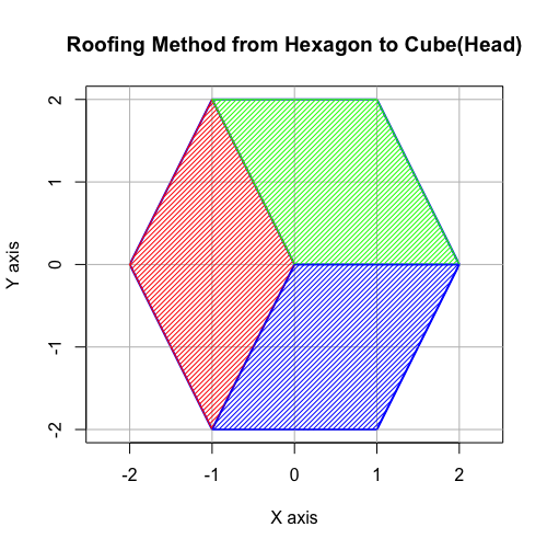
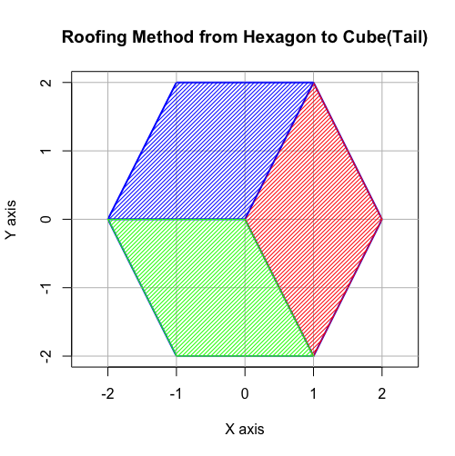
そして「屋根掛け法(Roofing Method)」による立方体や正八面体からの正十二面体への変換操作は2^n3^m集の構築する同心球面空間から2^n3^m5^l集の構築する同心球面空間への乗り換えという話になってきそうです。
【オイラーの多面体定理と正多面体】二次元上の多角形と三次元上の多面体の往復
体系統合(System Assemble)に不可欠な二辺形(Bilateral)への言及
こうした諸特徴/諸操作を体系統合(System Assemble)には二辺形(Bilateral)への言及が不可欠となります。
【Rで球面幾何学】何故「正方形」ではCos(θ)+Sin(θ)iが成立するのか?

とりあえず抑えておかなければいけない特徴は以下。
①正方形同様cos(θ)+sin(θ)(i)が通用する2^n集の同心円集合に含まれる。
【Rで九九】どうして36個の数字しか使われないのか?
【初心者向け】「単位円筒」から「単位球面」へ

②2個集めると円上に正方形を構成する(2^n集の同心円集合枠内での操作)。
【Rで球面幾何学】何故「正方形」ではCos(θ)+Sin(θ)iが成立するのか?

③3個集めると2^n3^m集の同心円集合に推移し、円上に六角形、球面上に正八面体を構成する。
【オイラーの多面体定理と正多面体】とある「球面幾何学(Spherical Geometry)」の出発点…
④また円上の六角形は「屋根掛け法(Roofing Method)」により立方体に推移する(2^n3^m集の同心円集合枠内での操作)。
【オイラーの多面体定理と正多面体】二次元上の多角形と三次元の多面体の往復
ここから、こういう集合関係が浮かび上がってくるのです。
- 2^n集…二辺形(Bilateral),正方形(Square)
- 3^n集…三角形(Triangle),四面体(Tetrahedron)
- 5^n集…五角形(Pentagon)
- 2^n3^m集…立方体(Cube),正八面体(Octahedron),六角形(Hexagon)
- 2^n3^m5^l集…正十二面体(Dodecahedron),正二十面体(Icosahedron)

library(gplots)

Set2<-c("Bilateral", "Square","Cube","Octahedron","Hexagon", "Dodecahedron","Icosahedron")
Set3<- c("Triangle","Tetrahedron","Cube","Octahedron","Hexagon","Dodecahedron","Icosahedron")
Set5 <- c("Pentagon","Dodecahedron","Icosahedron")
data <- list(x2_Set=Set2, x3_Set=Set3, x5_Set= Set5)

venn(data)

library(UpSetR)

Set2<-c("Bilateral", "Square","Cube","Octahedron","Hexagon", "Dodecahedron","Icosahedron")
Set3<- c("Triangle","Tetrahedron","Cube","Octahedron","Hexagon","Dodecahedron","Icosahedron")
Set5 <- c("Pentagon","Dodecahedron","Icosahedron")
data <- list(x2_Set=Set2, x3_Set=Set3, x5_Set= Set5)

upset(fromList(data), order.by = "freq")
こうして、なんとなく全体像が浮かび上がってきた所で以下続報…