CNTK 2.2 Python API 解説 (1) - CIFAR-10 CNN モデルの改良 / VGG, ResNet の実装
0. はじめに
◆ CNTK ( Microsoft Cognitive Toolkit ) 2.2 の Python API 解説第1弾です。
i.e. 本記事は CNTK 2.2 Python API 入門シリーズの続編となるシリーズ - 「解説シリーズ」の第1回の記事になります。
今回は畳み込みニューラルネットワークの中級レベル程度の内容を CNTK で実装します :
- CIFAR-10 を題材に、分類タスク用の基本的な CNN モデルを CNTK で作成します。
- ドロップアウト層やバッチ正規化層の追加により基本モデルを改良します。
- 更に、VGG スタイルのモデルや ResNet モデルも作成してみます。
(VGG / ResNet については簡単ですが直感的に分かりやすく説明しておきました。) - データリーダーとしては CNTK の Image Reader を利用し、それに合わせた前処理を行ないます。
◆ これまでに、CNTK 2.2 Python API について以下の記事を公開してきました :
- CNTK 2.2 Python API 入門 - (1) 基本, (2) 2 クラス分類, (3) MNIST, (4) LSTM, (5) オートエンコーダ (6) 総集編
- CNTK 2.2 Python API ガイド - 深層学習フレームワーク経験者のために
これらは主として CNTK 2.2 Tutorials の初級 (100 番台) と 200 番を参考にした入門レベルの記事ですが、
今回から始まる CNTK 2.2 Python API 解説シリーズはチュートリアルの中級 (200 番台) を参考にして記事を作成していきます。
想定している読者は、Python / 深層学習の基礎知識を持つことに加えて、CNTK にある程度は慣れていることが条件に追加されます。もちろん上記の入門シリーズに多少なりとも目を通していれば問題ありません。
基礎理論の冗長な説明は限定的ですので、例えば他のフレームワーク経験者の場合には、入門記事よりも読みやすくなるかと思います。

本記事の内容 :
- 動作環境と Jupyter Notebook について
- CIFAR-10 データセットの前処理
- 畳み込みニューラルネットワークと CNTK Python API
- 基本モデル
- VGG
- ResNet
- What's Next
本記事は以下のチュートリアルとリファレンスを参考にしています :
- CNTK 201: Part A - CIFAR-10 Data Loader
- CNTK 201: Part B - Image Understanding
- CNTK 103: Part A - MNIST Data Loader
- CNTK 103: Part D - Convolutional Neural Network with MNIST
- Layers Library Reference
1. 動作環境と Jupyter Notebook について
動作環境
動作環境の構築が必要な場合には、Cognitive Toolkit 2.2 を Azure Linux GPU 仮想マシンにインストール を参考にしてください。Azure ポータルと Ubuntu Linux にある程度慣れていれば、30 分程度で以下のような環境が構築できるかと思います :
- Azure NC 仮想マシン with NVIDIA Tesla® K80 GPU
- Ubuntu 16.04 LTS
- NVIDIA CUDA 8.0 & cuDNN 6.0
- Anaconda 3 4.1.1
- CNTK 2.2 (for GPU)
Jupyter Notebook
また、本記事でも CNTK チュートリアルでも Jupyter Notebook を多用します。
Jupyter Notebook の利用方法については「CNTK 2.2 Python API 入門 (2)」の記事中の Jupyter Notebook の活用 を参照してください。
2. CIFAR-10 データセットの前処理
この章では CNTK による画像分類タスクにおいて画像データをどのように準備するかを示します。
CNTK によりサポートされるフォーマットに変換してセーブし、4 章からの CNTK による分類タスクで実際に利用します。
今回は deserializer として (CTFDeserializer ではなく、) ImageDeserializer を利用します。
そのため、(MNIST の前処理では扱わなかった) ファイルも併せて生成する必要があります。
【参考】 CNTK CTF フォーマットによる前処理の詳細は: CNTK 2.2 Python API 入門 (3) - 2.MNIST データセットを CNTK CTF フォーマットでセーブする を参照してください。
データセットは有名な CIFAR-10 データセットを利用します。これは Alex Krizhevsky, Vinod Nair, そして Geoffrey Hinton により収集された画像分類のためのポピュラーなデータセットで、80 Million Tiny Images データセットのラベル付けられたサブセットです。
インポート
それでは始めます。まずは必要なコンポーネントをインポートします :
※ Jupyter Notebook の利用を想定しています。
from __future__ import print_function # Use a function definition from future version (say 3.x from 2.7 interpreter)

from PIL import Image
import getopt
import numpy as np
import pickle as cp
import os
import shutil
import struct
import sys
import tarfile
import xml.etree.cElementTree as et
import xml.dom.minidom

try:
    from urllib.request import urlretrieve
except ImportError:
    from urllib import urlretrieve

# Config matplotlib for inline plotting
%matplotlib inline
2-1 ダウンロードとセーブ
CIFAR-10 データセットは、クラス毎に 6,000 画像、10 クラスの 60,000 32x32 カラー画像から成ります。50,000 訓練画像と 10,000 テスト画像に分割されています。
10 クラスは :
airplane, automobile, bird, cat, deer, dog, frog, horse, ship, そして truck
データを読み込む際に必要な特徴次元を設定しておきます :
# CIFAR Image data
imgSize = 32
numFeature = imgSize * imgSize * 3
(1) 基本処理 (ダウンロードから CTF ファイルへのセーブ) のためのヘルパー関数
ダウンロードする CIFAR-10 のアーカイブは data_batch_1, data_batch_2, ..., data_batch_5, そして test_batch ファイルを含みます。ファイルの各々は cPickle により pickle 化された、つまりシリアライズされたオブジェクトです。
これらのファイルをアンパックして NumPy スタックを作成し、そして CTF フォーマットでセーブすることになります。
そのためのヘルパー関数を3つ定義します :
-
readBatch-loadDataから名前で渡される pickle ファイルを unpack します。 -
loadData- ファイルをダウンロードしたら解凍し、data_batch_1, data_batch_2, ..., data_batch_5 と test_batch ファイルを得ます。そしてreadBatchを利用してデータをロードして trn, tst 変数にストアします。 -
saveTxt- ラベルと特徴をテキストファイルにセーブします。
そのフォーマットは CTF フォーマットで、以下のような形式をしています。ラベルは one-hot エンコードされます :
|labels 0 0 0 0 0 0 1 0 0 0 |features 59 43 50 68 98 119 139 145 149 149 ...
def readBatch(src):
    with open(src, 'rb') as f:
        if sys.version_info[0] < 3:
            d = cp.load(f)
        else:
            d = cp.load(f, encoding='latin1')
        data = d['data']
        feat = data
    res = np.hstack((feat, np.reshape(d['labels'], (len(d['labels']), 1))))
    return res.astype(np.int)

def loadData(src):
    print ('Downloading ' + src)
    fname, h = urlretrieve(src, './delete.me')
    print ('Done.')
    try:
        print ('Extracting files...')
        with tarfile.open(fname) as tar:
            tar.extractall()
        print ('Done.')
        print ('Preparing train set...')
        trn = np.empty((0, numFeature + 1), dtype=np.int)
        for i in range(5):
            batchName = './cifar-10-batches-py/data_batch_{0}'.format(i + 1)
            trn = np.vstack((trn, readBatch(batchName)))
        print ('Done.')
        print ('Preparing test set...')
        tst = readBatch('./cifar-10-batches-py/test_batch')
        print ('Done.')
    finally:
        os.remove(fname)
    return (trn, tst)

def saveTxt(filename, ndarray):
    with open(filename, 'w') as f:
        labels = list(map(' '.join, np.eye(10, dtype=np.uint).astype(str)))
        for row in ndarray:
            row_str = row.astype(str)
            label_str = labels[row[-1]]
            feature_str = ' '.join(row_str[:-1])
            f.write('|labels {} |features {}\n'.format(label_str, feature_str))
(2) 画像フォーマットでもセーブする
ImageDeserializer を利用するために、画像を CTF テキストフォーマットでセーブするだけでなく、PNG フォーマットでも画像をセーブします。更に、画像の平均 (mean) も計算します。
saveImage と saveMean はこの目的のために使用される2つの関数です :
-
saveImageは個別の画像を処理しますが、単に画像を PNG でセーブするだけでなく、画像ファイル名からクラスへのマップ、チャネル毎の平均を正規化した値も書き出します。 -
saveMeanは画像全体に渡るピクセル毎の平均を CHW フォーマットで書き出します。
def saveImage(fname, data, label, mapFile, regrFile, pad, **key_parms):
    # data in CIFAR-10 dataset is in CHW format.
    pixData = data.reshape((3, imgSize, imgSize))
    if ('mean' in key_parms):
        key_parms['mean'] += pixData

    if pad > 0:
        pixData = np.pad(pixData, ((0, 0), (pad, pad), (pad, pad)), mode='constant', constant_values=128)

    img = Image.new('RGB', (imgSize + 2 * pad, imgSize + 2 * pad))
    pixels = img.load()
    for x in range(img.size[0]):
        for y in range(img.size[1]):
            pixels[x, y] = (pixData[0][y][x], pixData[1][y][x], pixData[2][y][x])
    img.save(fname)
    mapFile.write("%s\t%d\n" % (fname, label))

    # compute per channel mean and store for regression example
    channelMean = np.mean(pixData, axis=(1,2))
    regrFile.write("|regrLabels\t%f\t%f\t%f\n" % (channelMean[0]/255.0, channelMean[1]/255.0, channelMean[2]/255.0))

def saveMean(fname, data):
    root = et.Element('opencv_storage')
    et.SubElement(root, 'Channel').text = '3'
    et.SubElement(root, 'Row').text = str(imgSize)
    et.SubElement(root, 'Col').text = str(imgSize)
    meanImg = et.SubElement(root, 'MeanImg', type_id='opencv-matrix')
    et.SubElement(meanImg, 'rows').text = '1'
    et.SubElement(meanImg, 'cols').text = str(imgSize * imgSize * 3)
    et.SubElement(meanImg, 'dt').text = 'f'
    et.SubElement(meanImg, 'data').text = ' '.join(['%e' % n for n in np.reshape(data, (imgSize * imgSize * 3))])

    tree = et.ElementTree(root)
    tree.write(fname)
    x = xml.dom.minidom.parse(fname)
    with open(fname, 'w') as f:
        f.write(x.toprettyxml(indent = '  '))
saveTrainImages と saveTestImages はデータセットに渡りイテレートするための単なるラッパー関数です :
def saveTrainImages(filename, foldername):
    if not os.path.exists(foldername):
        os.makedirs(foldername)
    data = {}
    dataMean = np.zeros((3, imgSize, imgSize)) # mean is in CHW format.
    with open('train_map.txt', 'w') as mapFile:
        with open('train_regrLabels.txt', 'w') as regrFile:
            for ifile in range(1, 6):
                with open(os.path.join('./cifar-10-batches-py', 'data_batch_' + str(ifile)), 'rb') as f:
                    if sys.version_info[0] < 3:
                        data = cp.load(f)
                    else:
                        data = cp.load(f, encoding='latin1')
                    for i in range(10000):
                        fname = os.path.join(os.path.abspath(foldername), ('%05d.png' % (i + (ifile - 1) * 10000)))
                        saveImage(fname, data['data'][i, :], data['labels'][i], mapFile, regrFile, 4, mean=dataMean)
    dataMean = dataMean / (50 * 1000)
    saveMean('CIFAR-10_mean.xml', dataMean)

def saveTestImages(filename, foldername):
    if not os.path.exists(foldername):
      os.makedirs(foldername)
    with open('test_map.txt', 'w') as mapFile:
        with open('test_regrLabels.txt', 'w') as regrFile:
            with open(os.path.join('./cifar-10-batches-py', 'test_batch'), 'rb') as f:
                if sys.version_info[0] < 3:
                    data = cp.load(f)
                else:
                    data = cp.load(f, encoding='latin1')
                for i in range(10000):
                    fname = os.path.join(os.path.abspath(foldername), ('%05d.png' % i))
                    saveImage(fname, data['data'][i, :], data['labels'][i], mapFile, regrFile, 0)
URL やファイル名を定義しましょう :
# URLs for the train image and labels data
url_cifar_data = 'http://www.cs.toronto.edu/~kriz/cifar-10-python.tar.gz'

# Paths for saving the text files
data_dir = './data/CIFAR-10/'
train_filename = data_dir + '/Train_cntk_text.txt'
test_filename = data_dir + '/Test_cntk_text.txt'

train_img_directory = data_dir + '/Train'
test_img_directory = data_dir + '/Test'

root_dir = os.getcwd()
(3) ラベルと特徴をセーブする
さて、実行します。訓練とテストの両者についてラベルと特徴を CTF テキストファイルにセーブした後、各種ファイルを生成します :
if not os.path.exists(data_dir):
    os.makedirs(data_dir)

try:
    os.chdir(data_dir)
    trn, tst= loadData('https://www.cs.toronto.edu/~kriz/cifar-10-python.tar.gz')
    print ('Writing train text file...')
    saveTxt(r'./Train_cntk_text.txt', trn)
    print ('Done.')
    print ('Writing test text file...')
    saveTxt(r'./Test_cntk_text.txt', tst)
    print ('Done.')
    print ('Converting train data to png images...')
    saveTrainImages(r'./Train_cntk_text.txt', 'train')
    print ('Done.')
    print ('Converting test data to png images...')
    saveTestImages(r'./Test_cntk_text.txt', 'test')
    print ('Done.')
finally:
    os.chdir("../..")
Downloading https://www.cs.toronto.edu/~kriz/cifar-10-python.tar.gz
Done.
Extracting files...
Done.
Preparing train set...
Done.
Preparing test set...
Done.
Writing train text file...
Done.
Writing test text file...
Done.
Converting train data to png images...
Done.
Converting test data to png images...
Done.
2-2 生成ファイルの確認
生成されたファイルを確認してみましょう :
$ pwd
/home/masao/ws.cntk/data/CIFAR-10

$ ls -lFh
total 639M
drwxr-xr-x 2 masao masao 4.0K Jun  4  2009 cifar-10-batches-py/
-rw-rw-r-- 1 masao masao  40K Oct 29 14:23 CIFAR-10_mean.xml
drwxrwxr-x 2 masao masao 260K Oct 29 14:23 test/
-rw-rw-r-- 1 masao masao 106M Oct 29 14:21 Test_cntk_text.txt
-rw-rw-r-- 1 masao masao 596K Oct 29 14:23 test_map.txt
-rw-rw-r-- 1 masao masao 381K Oct 29 14:23 test_regrLabels.txt
drwxrwxr-x 2 masao masao 1.5M Oct 29 14:23 train/
-rw-rw-r-- 1 masao masao 526M Oct 29 14:21 Train_cntk_text.txt
-rw-rw-r-- 1 masao masao 3.0M Oct 29 14:23 train_map.txt
-rw-rw-r-- 1 masao masao 1.9M Oct 29 14:23 train_regrLabels.txt

# これはアーカイブを解凍したものです :
$ ls -lh cifar-10-batches-py/
total 178M
-rw-r--r-- 1 masao masao 158 Mar 31  2009 batches.meta
-rw-r--r-- 1 masao masao 30M Mar 31  2009 data_batch_1
-rw-r--r-- 1 masao masao 30M Mar 31  2009 data_batch_2
-rw-r--r-- 1 masao masao 30M Mar 31  2009 data_batch_3
-rw-r--r-- 1 masao masao 30M Mar 31  2009 data_batch_4
-rw-r--r-- 1 masao masao 30M Mar 31  2009 data_batch_5
-rw-r--r-- 1 masao masao  88 Jun  4  2009 readme.html
-rw-r--r-- 1 masao masao 30M Mar 31  2009 test_batch

# 画像ファイルです :
$ ls -lh train | head
total 196M
-rw-rw-r-- 1 masao masao 2.6K Oct 29 14:21 00000.png
-rw-rw-r-- 1 masao masao 2.8K Oct 29 14:21 00001.png
-rw-rw-r-- 1 masao masao 2.2K Oct 29 14:21 00002.png
-rw-rw-r-- 1 masao masao 2.5K Oct 29 14:21 00003.png
-rw-rw-r-- 1 masao masao 2.5K Oct 29 14:21 00004.png
-rw-rw-r-- 1 masao masao 2.7K Oct 29 14:21 00005.png
-rw-rw-r-- 1 masao masao 2.6K Oct 29 14:21 00006.png
-rw-rw-r-- 1 masao masao 2.7K Oct 29 14:21 00007.png
-rw-rw-r-- 1 masao masao 2.3K Oct 29 14:21 00008.png

$ ls -lh test | head
total 40M
-rw-rw-r-- 1 masao masao 2.5K Oct 29 14:23 00000.png
-rw-rw-r-- 1 masao masao 2.2K Oct 29 14:23 00001.png
-rw-rw-r-- 1 masao masao 2.3K Oct 29 14:23 00002.png
-rw-rw-r-- 1 masao masao 2.2K Oct 29 14:23 00003.png
-rw-rw-r-- 1 masao masao 2.6K Oct 29 14:23 00004.png
-rw-rw-r-- 1 masao masao 2.4K Oct 29 14:23 00005.png
-rw-rw-r-- 1 masao masao 2.5K Oct 29 14:23 00006.png
-rw-rw-r-- 1 masao masao 2.2K Oct 29 14:23 00007.png
-rw-rw-r-- 1 masao masao 2.4K Oct 29 14:23 00008.png
次にテキストファイルの内容を確認します。
まずは Train_cntk_text.txt と Test_cntk_text.txt です :
$ wc -l Train_cntk_text.txt Test_cntk_text.txt
    50000 Train_cntk_text.txt
    10000 Test_cntk_text.txt
    60000 total

$ head -n 1 Train_cntk_text.txt
|labels 0 0 0 0 0 0 1 0 0 0 |features 59 43 50 68 98 119 139 145 149 149 131 125 142 144 137 129 137 134 124 139 139 133 136 139 152 163 168 159 158 158 152 148 16 0 18 51 88 120 128 127 126 116 106 101 105 113 109 112 119 109 105 125 127 122 131 124 121 131 132 133 133 123 119 122 25 16 49 83 110 129 130 121 113 112 112 106 105 128 124 130 127 122 115 120 130 131 139 127 126 127 130 142 130 118 120 109 33 38 87 106 115 117 114 105 107 121 125 109 113 146 133 127 118 117 127 122 132 137 136 131 124 130 132 135 130 125 121 94 50 59 102 127 124 121 120 114 107 125 129 106 108 124 121 108 98 110 117 120 134 140 131 141 135 127 121 119 103 87 75 67 71 84 110 129 136 131 129 119 108 122 123 105 107 111 108 98 94 97 83 88 102 97 88 118 140 136 120 107 88 67 35 32 97 111 123 130 136 132 122 121 127 138 124 120 107 80 68 74 101 105 65 58 63 78 136 122 139 151 129 108 95 96 89 66 115 119 130 140 133 127 138 137 131 133 134 108 72 51 41 72 181 209 125 68 64 82 123 112 135 151 137 114 105 101 126 102 137 128 132 128 119 123 128 130 121 137 131 74 54 50 44 86 203 217 162 100 77 75 74 76 107 135 135 129 127 119 125 134 154 154 156 140 123 125 126 127 133 132 90 63 62 70 79 103 152 148 141 121 101 96 86 75 101 136 136 134 133 132 128 133 154 155 156 147 133 137 139 134 141 121 80 97 90 98 137 139 148 134 138 134 140 175 142 102 108 135 131 133 138 136 130 134 145 146 146 135 127 129 117 103 130 120 111 146 136 163 169 152 161 148 177 161 195 209 189 125 108 140 137 132 136 133 132 133 142 141 140 144 147 121 84 88 109 101 138 213 178 191 211 189 205 207 213 191 199 188 161 130 124 131 130 131 134 135 136 133 158 154 142 143 132 90 72 81 84 107 165 229 183 191 239 219 228 225 214 216 210 200 189 174 161 139 134 126 131 142 136 138 145 149 147 147 136 80 89 105 96 129 192 185 145 203 223 242 244 238 241 227 225 235 219 224 215 156 128 129 131 133 128 130 148 146 145 147 133 63 66 88 113 182 220 138 162 206 196 247 255 255 245 236 230 215 231 250 241 158 125 126 124 125 126 124 149 143 144 151 132 64 84 112 163 223 206 145 196 204 220 243 245 239 234 231 195 150 208 250 227 163 145 143 140 136 121 114 147 134 140 148 135 100 108 144 210 248 175 175 220 226 230 233 224 201 184 181 190 170 179 231 223 162 146 140 139 145 142 128 152 117 114 123 126 122 93 179 238 248 170 185 241 230 187 180 166 146 149 157 184 216 212 236 236 166 136 134 130 127 137 151 145 127 128 133 132 135 171 237 252 229 173 169 220 194 123 135 127 151 165 132 151 202 240 240 222 156 119 120 112 100 99 140 143 127 129 129 130 140 219 244 210 193 166 153 191 179 128 147 149 172 147 128 141 173 202 190 198 152 100 109 119 121 108 136 143 125 131 128 123 153 148 166 188 182 171 165 195 190 152 143 152 153 142 141 135 136 148 141 141 138 111 111 121 129 138 179 141 131 139 139 138 151 128 136 175 173 189 205 201 168 151 145 146 149 153 149 144 144 145 143 129 123 124 113 108 113 148 199 143 139 138 149 160 150 147 151 169 167 179 212 203 207 149 139 144 137 151 155 152 140 107 91 84 105 132 118 96 102 159 190 149 133 136 147 150 153 157 162 175 190 166 202 224 197 192 180 146 126 141 156 153 115 77 79 93 126 133 119 113 140 187 154 172 144 135 136 135 139 153 163 166 184 166 150 184 156 158 168 149 135 130 132 128 127 135 143 139 136 127 121 135 189 211 136 202 187 151 128 122 134 142 150 153 148 135 127 153 166 143 130 128 151 152 135 139 155 161 154 154 143 130 132 171 215 186 117 216 193 168 151 131 126 138 144 142 137 120 131 145 144 137 127 126 139 153 149 140 135 147 148 149 149 137 143 203 206 124 71 220 201 186 172 156 142 142 153 150 139 126 136 148 141 131 126 127 138 150 154 149 124 126 141 145 147 127 114 186 173 56 33 208 201 198 191 183 171 159 147 135 130 139 147 144 145 137 136 137 148 152 150 155 138 120 128 142 135 90 50 137 160 56 53 180 173 186 194 198 201 189 173 156 139 142 145 141 141 139 140 143 139 138 143 146 135 117 112 122 104 58 34 131 184 97 83 177 168 179 188 202 218 218 207 191 175 166 163 163 161 153 159 162 149 140 148 161 144 112 119 130 120 92 103 170 216 151 123 62 46 48 54 73 91 107 110 117 120 103 99 115 112 105 97 106 106 97 113 112 105 105 108 120 131 136 129 130 132 125 124 20 0 8 27 51 82 89 86 87 79 70 67 70 74 70 72 79 71 69 89 92 85 89 82 79 89 91 94 96 88 83 87 24 7 27 50 72 92 93 82 77 78 79 75 73 92 87 92 89 85 79 85 95 96 102 90 89 89 92 105 94 84 84 73 25 20 54 63 70 74 72 62 68 84 90 75 77 105 91 84 76 76 87 81 92 99 99 93 86 91 90 93 90 87 85 62 32 32 65 79 77 77 78 74 72 88 89 68 71 83 78 68 65 74 80 80 93 106 95 98 92 84 79 79 67 57 47 42 48 53 73 82 88 84 84 77 70 82 81 65 72 77 74 65 62 63 56 58 68 69 54 74 96 97 80 68 54 39 10 13 69 75 85 84 88 83 74 74 83 94 79 79 71 50 43 41 51 56 37 36 37 51 93 68 86 106 87 68 59 63 61 47 82 76 90 97 88 81 90 89 86 89 91 70 39 26 22 31 102 127 76 40 38 53 77 56 81 103 95 76 69 66 92 74 100 82 91 87 81 82 85 85 80 97 94 42 25 29 29 39 106 109 90 58 42 43 39 35 67 96 97 91 89 83 86 95 120 112 114 100 89 86 86 91 97 97 60 35 33 39 50 53 70 64 79 75 58 54 48 38 63 91 92 93 93 93 86 92 122 117 117 108 100 100 102 102 111 87 40 53 45 56 91 84 87 73 82 85 92 129 99 61 67 90 87 91 97 95 86 93 114 109 109 97 92 94 84 74 103 83 60 86 78 116 115 100 116 97 121 110 150 167 146 78 63 96 95 93 95 90 87 92 115 106 105 105 110 89 56 61 80 57 79 150 123 150 169 148 164 162 164 143 158 151 121 83 77 87 91 93 93 91 89 91 131 119 107 102 92 59 44 52 47 55 106 176 137 158 216 192 188 188 177 174 171 169 162 137 118 95 96 90 92 98 89 97 115 109 108 105 95 47 57 68 51 81 152 148 101 162 200 227 227 220 219 197 191 209 206 208 192 118 89 95 95 97 89 92 116 100 100 100 96 42 43 50 65 146 191 94 105 156 166 234 253 252 234 217 208 196 217 241 229 132 95 97 92 91 88 88 115 95 97 99 87 40 59 69 121 204 182 90 133 157 188 226 237 233 224 217 181 137 193 241 216 142 127 129 123 116 95 82 111 88 99 103 89 64 73 104 181 243 147 119 176 197 207 218 212 186 163 158 171 157 167 218 206 133 116 115 116 123 119 102 114 75 80 90 91 83 58 154 226 243 134 132 214 218 169 160 146 119 116 124 157 195 198 221 212 125 85 81 83 86 105 128 105 82 90 92 89 95 145 227 247 213 136 121 182 169 89 98 91 114 127 99 126 183 228 225 196 117 76 75 66 65 74 121 104 80 86 85 86 102 196 232 199 173 129 104 146 145 86 102 106 131 108 94 113 150 183 171 175 124 72 81 88 92 82 119 104 76 85 81 81 117 118 141 166 156 134 115 148 153 108 95 105 110 102 102 101 101 110 106 111 113 100 111 118 116 116 162 102 80 89 87 90 111 91 97 136 136 151 160 157 131 108 97 101 106 110 108 104 105 104 102 96 103 126 135 133 122 136 184 103 87 89 96 109 106 104 104 121 123 141 174 168 177 112 96 102 94 107 111 109 101 76 60 61 99 142 141 121 113 149 174 107 80 88 99 104 109 112 117 131 145 124 168 197 175 165 144 106 82 97 112 109 74 43 50 73 117 134 116 99 121 165 132 128 88 85 88 90 94 108 117 120 136 118 110 149 121 123 130 109 91 85 88 84 83 92 105 108 112 105 92 102 159 181 107 157 129 100 79 76 88 98 106 106 99 87 82 109 121 99 88 87 108 106 90 95 110 113 107 112 105 93 90 131 183 155 86 174 136 122 111 88 82 94 100 95 92 78 87 99 101 94 83 82 94 108 104 95 91 103 105 108 109 101 107 167 173 93 48 182 150 148 139 120 103 100 108 105 98 88 92 102 101 89 82 81 88 100 104 101 78 85 101 107 112 101 87 155 144 29 19 170 153 161 157 146 135 121 107 95 87 93 98 95 99 91 89 90 102 106 103 110 94 76 84 102 103 69 24 105 133 31 34 139 123 144 153 158 164 153 137 118 99 97 97 92 93 91 91 95 99 98 96 93 84 80 72 81 67 31 5 94 148 62 53 144 129 142 149 168 189 191 181 163 143 132 128 127 123 114 120 124 116 104 103 105 95 90 91 96 87 67 78 140 184 118 92 63 45 43 42 52 63 75 80 89 93 77 76 91 86 79 71 79 76 64 78 75 69 74 77 89 100 108 102 104 108 102 103 20 0 0 8 21 43 45 44 50 44 37 35 36 35 33 37 44 33 27 46 46 39 47 41 37 48 53 58 60 55 50 57 21 0 8 23 41 54 55 47 43 44 46 45 38 48 47 56 56 51 43 47 54 55 62 51 49 50 53 68 58 50 50 42 17 4 25 28 33 35 37 33 33 45 53 40 38 58 47 45 40 41 52 43 51 58 57 52 44 50 49 51 50 50 48 35 21 11 34 39 36 36 40 39 34 49 51 31 33 42 39 29 23 37 49 41 50 66 58 66 51 45 41 40 32 27 23 25 29 24 37 38 45 42 43 37 33 44 39 25 31 31 34 27 21 32 38 36 42 46 36 72 79 64 45 34 24 15 0 4 40 36 43 38 44 40 30 31 46 54 34 39 34 14 17 17 21 23 16 19 18 31 83 80 79 69 49 36 29 37 38 30 49 33 47 53 48 40 47 46 48 46 46 39 19 10 14 17 69 81 47 23 17 30 62 55 60 61 54 39 34 33 59 46 68 41 51 48 44 43 44 44 40 54 53 20 16 16 18 15 56 62 71 49 27 24 24 22 36 59 58 49 48 43 45 56 89 77 82 65 53 50 48 52 60 68 30 9 16 20 30 26 33 37 61 57 41 33 24 21 32 53 53 50 52 52 45 55 94 82 82 70 64 66 68 66 81 68 13 17 17 30 57 49 54 37 46 57 76 106 53 26 25 41 45 51 57 55 46 57 89 73 69 55 57 65 55 42 70 55 14 22 23 77 69 52 73 57 82 71 113 123 94 40 25 52 59 56 57 51 46 56 86 69 68 64 74 65 34 33 44 23 19 59 41 98 122 99 110 115 118 91 97 88 76 50 38 51 61 60 57 52 48 56 98 82 74 65 59 36 22 24 19 25 50 92 57 103 176 149 128 120 112 112 110 109 114 100 76 57 66 59 56 60 48 61 79 66 68 65 62 21 32 40 26 45 113 107 51 121 170 196 186 165 163 144 139 157 164 181 156 78 57 62 60 60 50 56 79 54 55 51 54 21 31 34 37 110 169 71 63 112 135 212 232 219 197 180 170 160 197 229 195 78 49 58 52 49 46 54 79 49 51 51 49 21 41 37 75 166 157 56 84 110 156 208 226 215 201 192 152 100 154 216 173 78 60 62 55 46 30 40 76 47 61 66 60 38 43 66 140 212 115 73 129 164 179 196 195 166 138 128 136 105 105 181 161 71 43 34 33 38 35 41 80 37 48 57 56 48 32 138 212 229 104 88 177 195 142 131 115 85 79 83 110 141 152 197 176 63 16 13 13 16 27 54 72 41 51 53 49 51 110 205 235 194 100 73 138 135 55 60 48 63 74 50 79 142 203 210 169 64 12 16 14 15 19 54 66 38 49 46 45 59 161 210 186 151 92 55 96 105 47 58 59 78 54 45 67 112 160 147 146 86 26 34 43 50 36 50 64 32 48 43 39 76 85 118 147 132 99 69 99 110 66 49 56 58 51 54 55 60 74 65 68 71 37 31 35 39 45 83 65 35 46 44 50 71 52 61 104 107 118 120 113 89 65 53 52 57 61 61 59 59 59 60 48 39 30 14 8 10 44 102 72 44 42 52 72 64 58 57 81 87 105 138 132 141 74 55 56 47 61 65 63 55 38 34 23 25 34 20 4 9 63 99 74 37 48 59 63 62 67 78 96 107 84 133 168 148 133 107 64 40 52 66 61 29 14 25 33 47 39 31 24 42 91 75 76 18 35 48 45 49 68 83 82 100 88 75 110 86 87 92 71 51 43 43 37 36 52 66 62 52 39 39 44 87 114 58 82 26 25 34 41 49 53 56 58 63 59 44 60 77 59 51 52 70 65 48 50 63 65 63 67 54 44 46 70 106 91 48 87 16 19 35 34 35 49 53 53 51 34 41 52 57 54 48 51 60 69 63 53 46 57 59 62 63 54 57 102 105 49 26 91 22 24 28 26 30 51 75 73 57 38 47 62 60 51 49 51 52 60 65 60 36 41 55 61 68 59 46 98 87 9 9 96 34 26 27 34 32 42 52 49 46 57 62 55 57 51 52 54 58 60 61 64 46 33 39 58 62 40 11 60 70 7 20 96 42 30 25 34 36 32 32 38 38 49 56 52 52 51 53 58 60 60 56 43 33 38 29 39 30 11 0 57 94 34 34 116 94 87 67 68 76 72 70 79 82 86 92 94 92 84 90 93 91 83 77 69 55 59 58 65 59 46 57 104 140 84 72
続いてマップファイルです :
$ head -n 10 train_map.txt
/home/masao/ws.cntk/data/CIFAR-10/train/00000.png     6
/home/masao/ws.cntk/data/CIFAR-10/train/00001.png     9
/home/masao/ws.cntk/data/CIFAR-10/train/00002.png     9
/home/masao/ws.cntk/data/CIFAR-10/train/00003.png     4
/home/masao/ws.cntk/data/CIFAR-10/train/00004.png     1
/home/masao/ws.cntk/data/CIFAR-10/train/00005.png     1
/home/masao/ws.cntk/data/CIFAR-10/train/00006.png     2
/home/masao/ws.cntk/data/CIFAR-10/train/00007.png     7
/home/masao/ws.cntk/data/CIFAR-10/train/00008.png     8
/home/masao/ws.cntk/data/CIFAR-10/train/00009.png     3
$ head -n 10 test_map.txt
/home/masao/ws.cntk/data/CIFAR-10/test/00000.png      3
/home/masao/ws.cntk/data/CIFAR-10/test/00001.png      8
/home/masao/ws.cntk/data/CIFAR-10/test/00002.png      8
/home/masao/ws.cntk/data/CIFAR-10/test/00003.png      0
/home/masao/ws.cntk/data/CIFAR-10/test/00004.png      6
/home/masao/ws.cntk/data/CIFAR-10/test/00005.png      6
/home/masao/ws.cntk/data/CIFAR-10/test/00006.png      1
/home/masao/ws.cntk/data/CIFAR-10/test/00007.png      6
/home/masao/ws.cntk/data/CIFAR-10/test/00008.png      3
/home/masao/ws.cntk/data/CIFAR-10/test/00009.png      1
そして各画像のチャネル毎の平均値を保持するファイル :
$ wc -l train_regrLabels.txt test_regrLabels.txt
  50000 train_regrLabels.txt
  10000 test_regrLabels.txt
  60000 total

$ head -n 10 train_regrLabels.txt
|regrLabels     0.535103        0.444485        0.341426
|regrLabels     0.507480        0.507897        0.508179
|regrLabels     0.515725        0.519912        0.513468
|regrLabels     0.431635        0.389721        0.324804
|regrLabels     0.411662        0.437711        0.471850
|regrLabels     0.538203        0.358350        0.325718
|regrLabels     0.483216        0.564495        0.394988
|regrLabels     0.513135        0.518963        0.426338
|regrLabels     0.454689        0.572831        0.655017
|regrLabels     0.376814        0.360316        0.335801

$ head -n 10 test_regrLabels.txt
|regrLabels     0.431468        0.434383        0.409279
|regrLabels     0.590725        0.604439        0.629665
|regrLabels     0.474606        0.522254        0.562776
|regrLabels     0.596392        0.590407        0.634482
|regrLabels     0.423009        0.478669        0.361489
|regrLabels     0.530258        0.345734        0.274724
|regrLabels     0.416590        0.243765        0.229316
|regrLabels     0.385880        0.384218        0.250551
|regrLabels     0.680189        0.633119        0.566199
|regrLabels     0.541153        0.533253        0.621706
画像全体のピクセル毎の平均値を保持するファイル :
$ cat CIFAR-10_mean.xml
<?xml version="1.0" ?>
<opencv_storage>
  <Channel>3</Channel>
  <Row>32</Row>
  <Col>32</Col>
  <MeanImg type_id="opencv-matrix">
    <rows>1</rows>
    <cols>3072</cols>
    <dt>f</dt>
    <data>1.307107e+02 1.301404e+02 1.310504e+02 1.315689e+02 1.321847e+02 ... 1.138641e+02 1.138778e+02 1.138306e+02 1.139062e+02 1.143819e+02</data>
  </MeanImg>
</opencv_storage>
3. 畳み込みニューラルネットワークと CNTK Python API
この章では (4 章以後に必要な) 畳み込みニューラルネットワークの基本的な層と、それに対応する CNTK Python API の簡単なおさらいをしておきます。
【参考】 CNTK における畳み込みニューラルネットワークの詳細は: CNTK 2.2 Python API 入門 (3) - 6. 畳み込みニューラルネットワークで MNIST を分類 を参照してください。
畳み込みニューラルネットワークはある層の出力が次の層に供給されるような多くの層から構成される順伝播ネットワークです。
(層をスキップするようなより複雑なアーキテクチャもありますが、それらの一つ (ResNet) については最後に扱います。)
通常、ネットワークは交互に続く畳み込み層とプーリング層で開始され、分類パートのための完全結合層で終わります。
3-1 畳み込み層
畳み込み層は、入力画像か前の層の出力に適用される複数の 2D 畳み込みカーネルから成り、各畳み込みカーネルは特徴マップを出力します。
※ ここで新しい Jupyter Notebook を作成してください :
from IPython.display import Image
Image(url="https://cntk.ai/jup/201/Conv2D.png")

特徴マップ出力のスタックは次の層への入力になります :
Image(url="https://cntk.ai/jup/201/Conv2DFeatures.png")

CNTK Python API:
Python API における畳み込み層は Convolution() です :
def Convolution(filter_shape,        # e.g. (3,3)
                num_filters,         # e.g. 64
                activation,          # relu or None...etc.
                init,                # Random initialization
                pad,                 # True or False
                strides)             # strides e.g. (1,1)
3-2 プーリング層
殆どの CNN ビジョン・アーキテクチャでは、各畳み込み層はプーリング層により継承され、それらは交互に完全結合層まで続きます。
プーリング層の目的は次のようなものです :
- 前の層の次元を削減します、これはネットワークを高速化します。
- 限定的な、変換の不変性を提供します。
下図はストライド 2 のマックスプーリングの例です :
Image(url="https://cntk.ai/jup/201/MaxPooling.png", width=400, height=400)

CNTK Python API:
Python API におけるプーリング層は MaxPooling(), AveragePooling() です :
# Max pooling
def MaxPooling(filter_shape,  # e.g. (3,3)
               strides,       # (2,2)
               pad)           # True or False

# Average pooling
def AveragePooling(filter_shape,  # e.g. (3,3)
                   strides,       # (2,2)
                   pad)           # True or False
- 通常はマックス・プーリングが使用されます。
- CNTK ではデフォルトで GlobalMaxPooling(), GlobalAveragePooling() も実装されています。GlobalAveragePooling はモデルによっては比較的良く利用されます。
3-3 ドロップアウト層
ドロップアウト層は入力として確率値を取り、この値はドロップアウト率と呼ばれます。
ドロップアウト率を 0.5 としましょう、この層が行なうことは前の層からのノードの 50 % を無作為に選択してネットワークからそれらをドロップアウト(脱落)させることです。この挙動はネットワークを正則化する助けとなります。
ドロップアウト: ニューラルネットワークがオーバーフィッティングを回避するための単純な方法です。
Nitish Srivastava, Geoffrey Hinton, Alex Krizhevsky, Ilya Sutskever, Ruslan Salakhutdinov
CNTK Python API:
Python API におけるドロップアウト層は Dropout() です :
# Dropout
def Dropout(prob)    # dropout rate e.g. 0.5
3-4 バッチ正規化 (BN)
バッチ正規化は各層への入力をバッチ単位で正規化 - 平均ゼロと分散 1 を持つようにする方法です。
BN はネットワークがより速く収束をする助けとなり各層の入力をゼロまわりに保持します。BN は gamma と beta と呼ばれる2つの学習可能なパラメータを持ち、これらのパラメータの目的はネットワークに正規化された入力がベストであるか生入力かを自身で決定させることです。
バッチ正規化: 内部的な共変量シフト (Internal Covariate Shift) を減少させることによって深層学習を加速します。
Sergey Ioffe, Christian Szegedy
CNTK Python API:
Python API におけるバッチ正規化層は BatchNormalization() です :
# Batch normalization
def BatchNormalization(map_rank)  # For image map_rank=1
4. 基本モデル
4-1 データセット
本章から CNN モデルの実装に入ります。
トレーニングするエポック数は環境やお好みに合わせて調整した上で、トレーニングを実行してください。
まずは題材である CIFAR-10 データセットを再確認しておきます :
Image(url="https://cntk.ai/jup/201/cifar-10.png", width=500, height=500)
上の画像は https://www.cs.toronto.edu/~kriz/cifar.html からのものです。
| ラベル | カテゴリー名 |
|---|---|
| 0 | airplane |
| 1 | automobile |
| 2 | bird |
| 3 | cat |
| 4 | deer |
| 5 | dog |
| 6 | frog |
| 7 | horse |
| 8 | ship |
| 9 | truck |
4-2 準備
必要なモジュールをインポートすることから始めます :
from __future__ import print_function # Use a function definition from future version (say 3.x from 2.7 interpreter)

import matplotlib.pyplot as plt
import math
import numpy as np
import os
import PIL
import sys
try:
    from urllib.request import urlopen
except ImportError:
    from urllib import urlopen

import cntk as C

%matplotlib inline
※ 次のブロックはチュートリアルからのそのままの引用です。
一般的には意味がないように思われますが、そのような環境が公開されているケースもあるかもしれませんので、このコードブロックも残しておきます (害はありません) :
下のブロックでは、環境変数を見て Notebook が CNTK 内部テストマシンで実行しているかを確認するものです。
そしてこの Notebook をテストするための正しいターゲットデバイス (GPU vs CPU) を選択します。
それ以外の場合には、ベストな利用可能デバイス (GPU, if available, else CPU) を使用するために CNTK のデフォルト・ポリシーを使用します :
if 'TEST_DEVICE' in os.environ:
    if os.environ['TEST_DEVICE'] == 'cpu':
        C.device.try_set_default_device(C.device.cpu())
    else:
        C.device.try_set_default_device(C.device.gpu(0))
4-3 データリーディング
モデルを訓練するためには2つのことが必要です :
- 訓練画像と相当するラベルを読む。
- コスト関数を定義し、各ミニバッチに対してコストを計算してそのコスト値に従ってモデルの重みを更新する。
◆ CNTK でデータを読むためには、CNTK リーダーを使用します。これはデータ拡張を可能にしてデータを並列に取得できます。
deserializer としては ImageDeserializer を利用します :
-
ImageDeserializer- 次の形式のファイルから画像と対応するラベルを読む画像リーダーを構成します :
<full path to image> <tab> <numerical label (0-based class id)>
このファイルは 2 章で作成済みです。マップ・テキストファイルは以下のような内容でした :
/home/masao/ws.cntk/data/CIFAR-10/train/00000.png     6
/home/masao/ws.cntk/data/CIFAR-10/train/00001.png     9
/home/masao/ws.cntk/data/CIFAR-10/train/00002.png     9
/home/masao/ws.cntk/data/CIFAR-10/train/00003.png     4
/home/masao/ws.cntk/data/CIFAR-10/train/00004.png     1
/home/masao/ws.cntk/data/CIFAR-10/train/00005.png     1
/home/masao/ws.cntk/data/CIFAR-10/train/00006.png     2
/home/masao/ws.cntk/data/CIFAR-10/train/00007.png     7
/home/masao/ws.cntk/data/CIFAR-10/train/00008.png     8
/home/masao/ws.cntk/data/CIFAR-10/train/00009.png     3
さて、create_reader() 関数を定義します。
特に難しい話しはありませんが、transforms リストは (入力データの前処理としての) 画像データ変換のための仕様リストであることに注意しましょう。
訓練時にはデータ拡張 (crop) も行なっています。
※ 環境変数 CNTK_EXTERNAL_TESTDATA_SOURCE_DIRECTORY については気にする必要はありません。
# Determine the data path for testing
# Check for an environment variable defined in CNTK's test infrastructure
envvar = 'CNTK_EXTERNAL_TESTDATA_SOURCE_DIRECTORY'
def is_test(): return envvar in os.environ

if is_test():
    data_path = os.path.join(os.environ[envvar],'Image','CIFAR','v0','tutorial201')
    data_path = os.path.normpath(data_path)
else:
    data_path = os.path.join('data', 'CIFAR-10')

# モデル次元
image_height = 32
image_width  = 32
num_channels = 3
num_classes  = 10

import cntk.io.transforms as xforms
#
# 訓練と評価の両者のためのリーダーを定義します。
#
def create_reader(map_file, mean_file, train):
    print("Reading map file:", map_file)
    print("Reading mean file:", mean_file)

    if not os.path.exists(map_file) or not os.path.exists(mean_file):
        raise RuntimeError("This tutorials depends 201A tutorials, please run 201A first.")

    # 特徴のための変換パイプラインは訓練時のみ jitter/crop を持ちます。
    transforms = []
    # 訓練はデータ拡張を使用します。
    if train:
        transforms += [
            xforms.crop(crop_type='randomside', side_ratio=0.8)
        ]
    transforms += [
        xforms.scale(width=image_width, height=image_height, channels=num_channels, interpolations='linear'),
        xforms.mean(mean_file)
    ]
    # deserializer
    return C.io.MinibatchSource(C.io.ImageDeserializer(map_file, C.io.StreamDefs(
        features = C.io.StreamDef(field='image', transforms=transforms), # マップ・ファイルの最初のカラムは 'image' として参照されます。
        labels   = C.io.StreamDef(field='label', shape=num_classes)      # そして2番目は 'label' として。
    )))
# 訓練とテスト・リーダーを作成します。
reader_train = create_reader(os.path.join(data_path, 'train_map.txt'),
                             os.path.join(data_path, 'CIFAR-10_mean.xml'), True)
reader_test  = create_reader(os.path.join(data_path, 'test_map.txt'),
                             os.path.join(data_path, 'CIFAR-10_mean.xml'), False)
Reading map file: data/CIFAR-10/train_map.txt
Reading mean file: data/CIFAR-10/CIFAR-10_mean.xml
Reading map file: data/CIFAR-10/test_map.txt
Reading mean file: data/CIFAR-10/CIFAR-10_mean.xml
Image(url="https://cntk.ai/jup/201/CNN.png")

4-4 基本モデル作成
必要な準備ができましたので、上図で示される基本的な CNN モデルを作成します :
- 畳み込み層とマックスプーリング層の組み合わせブロックを3つスタックします。
- 畳み込みカーネルは (5, 5) と少し大きめで、カーネル数は 32, 32, 64 です。
- 活性化関数は
relu。 - 重みは
C.glorot_uniform()で初期化されます。
ネットワークを CNTK 層 API を使用して実装します。with ブロックの利用により簡潔に記述できます :
def create_basic_model(input, out_dims):
    with C.layers.default_options(init=C.glorot_uniform(), activation=C.relu):
        net = C.layers.Convolution((5,5), 32, pad=True)(input)
        net = C.layers.MaxPooling((3,3), strides=(2,2))(net)

        net = C.layers.Convolution((5,5), 32, pad=True)(net)
        net = C.layers.MaxPooling((3,3), strides=(2,2))(net)

        net = C.layers.Convolution((5,5), 64, pad=True)(net)
        net = C.layers.MaxPooling((3,3), strides=(2,2))(net)

        net = C.layers.Dense(64)(net)
        net = C.layers.Dense(out_dims, activation=None)(net)

    return net
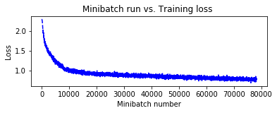
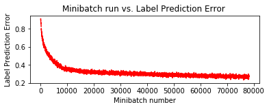
4-5 トレーニングと評価
さて、トレーニングと評価ループを書きましょう。
MNIST で使用した train_test() の定義と殆ど変わりありませんが、損失とエラーの進捗のグラフによる可視化も併せて行なっています :
- 入力特徴は正規化します。
- learner は
momentum_sgdを使用しています。 -
minibatch_sizeは 64 です。
#
# ネットワークを訓練して評価します。
#
def train_and_evaluate(reader_train, reader_test, max_epochs, model_func):
# 特徴とラベルデータを表す入力変数。
input_var = C.input_variable((num_channels, image_height, image_width))
label_var = C.input_variable((num_classes))
# 入力を正規化します。
feature_scale = 1.0 / 256.0
input_var_norm = C.element_times(feature_scale, input_var)
# 入力にモデルを適用します。
z = model_func(input_var_norm, out_dims=10)
#
# 訓練アクション
#
# 損失とメトリクス
ce = C.cross_entropy_with_softmax(z, label_var)
pe = C.classification_error(z, label_var)
# 訓練 config
epoch_size = 50000
minibatch_size = 64
# 訓練パラメータを設定します。
lr_per_minibatch = C.learning_rate_schedule([0.01]*10 + [0.003]*10 + [0.001],
C.UnitType.minibatch, epoch_size)
momentum_time_constant = C.momentum_as_time_constant_schedule(-minibatch_size/np.log(0.9))
l2_reg_weight = 0.001
# trainer オブジェクト
learner = C.momentum_sgd(z.parameters,
lr = lr_per_minibatch,
momentum = momentum_time_constant,
l2_regularization_weight=l2_reg_weight)
progress_printer = C.logging.ProgressPrinter(tag='Training', num_epochs=max_epochs)
trainer = C.Trainer(z, (ce, pe), [learner], [progress_printer])
# リーダー・ストリームからネットワーク入力へのマッピングを定義します。
input_map = {
input_var: reader_train.streams.features,
label_var: reader_train.streams.labels
}
C.logging.log_number_of_parameters(z) ; print()
# モデル訓練を遂行します。
batch_index = 0
plot_data = {'batchindex':[], 'loss':[], 'error':[]}
for epoch in range(max_epochs): # エポック数に渡るループ
sample_count = 0
while sample_count < epoch_size: # 各エポックにおけるミニバッチに渡るループ
data = reader_train.next_minibatch(min(minibatch_size, epoch_size - sample_count),
input_map=input_map) # fetch minibatch.
trainer.train_minibatch(data) # それでモデルを更新します。
sample_count += data[label_var].num_samples # ここまでに処理したサンプルをカウントします。
# 可視化のために...
plot_data['batchindex'].append(batch_index)
plot_data['loss'].append(trainer.previous_minibatch_loss_average)
plot_data['error'].append(trainer.previous_minibatch_evaluation_average)
batch_index += 1
trainer.summarize_training_progress()
#
# 評価アクション
#
epoch_size = 10000
minibatch_size = 16
# process minibatches and evaluate the model
metric_numer = 0
metric_denom = 0
sample_count = 0
minibatch_index = 0
while sample_count < epoch_size:
current_minibatch = min(minibatch_size, epoch_size - sample_count)
# 次のテスト・ミニバッチを取得します。
data = reader_test.next_minibatch(current_minibatch, input_map=input_map)
# minibatch data to be trained with
metric_numer += trainer.test_minibatch(data) * current_minibatch
metric_denom += current_minibatch
# ここまでに処理されたサンプル数を追跡します。
sample_count += data[label_var].num_samples
minibatch_index += 1
print("")
print("Final Results: Minibatch[1-{}]: errs = {:0.1f}% * {}".format(minibatch_index+1, (metric_numer*100.0)/metric_denom, metric_denom))
print("")
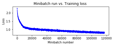
# 訓練結果を可視化します :
window_width = 32
loss_cumsum = np.cumsum(np.insert(plot_data['loss'], 0, 0))
error_cumsum = np.cumsum(np.insert(plot_data['error'], 0, 0))
# 移動平均
plot_data['batchindex'] = np.insert(plot_data['batchindex'], 0, 0)[window_width:]
plot_data['avg_loss'] = (loss_cumsum[window_width:] - loss_cumsum[:-window_width]) / window_width
plot_data['avg_error'] = (error_cumsum[window_width:] - error_cumsum[:-window_width]) / window_width
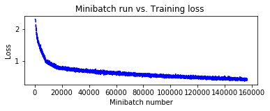
plt.figure(1)
plt.subplot(211)
plt.plot(plot_data["batchindex"], plot_data["avg_loss"], 'b--')
plt.xlabel('Minibatch number')
plt.ylabel('Loss')
plt.title('Minibatch run vs. Training loss ')
plt.show()
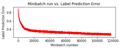
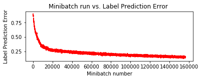
plt.subplot(212)
plt.plot(plot_data["batchindex"], plot_data["avg_error"], 'r--')
plt.xlabel('Minibatch number')
plt.ylabel('Label Prediction Error')
plt.title('Minibatch run vs. Label Prediction Error ')
plt.show()
return C.softmax(z)
◆ 前節で定義した、最も基本的なモデルを取り敢えず 100 エポックで訓練してみましょう :
※ Tesla K80 を使用しています。環境によってはエポック数を調整してください。
※ %%time はセル内のコードブロックの実行時間を計測するためのコマンドです。
%%time
pred = train_and_evaluate(reader_train,
                          reader_test,
                          max_epochs=100,
                          model_func=create_basic_model)
Training 116906 parameters in 10 parameter tensors.

Learning rate per minibatch: 0.01
Momentum per 1 samples: 0.9983550962823424
Finished Epoch[1 of 100]: [Training] loss = 2.071485 * 50000, metric = 76.96% * 50000 75.687s (660.6 samples/s);
Finished Epoch[2 of 100]: [Training] loss = 1.695251 * 50000, metric = 62.92% * 50000 6.931s (7214.0 samples/s);
Finished Epoch[3 of 100]: [Training] loss = 1.543050 * 50000, metric = 56.43% * 50000 6.834s (7316.4 samples/s);
Finished Epoch[4 of 100]: [Training] loss = 1.442975 * 50000, metric = 52.47% * 50000 6.723s (7437.2 samples/s);
Finished Epoch[5 of 100]: [Training] loss = 1.362026 * 50000, metric = 49.07% * 50000 6.851s (7298.2 samples/s);
Finished Epoch[6 of 100]: [Training] loss = 1.290451 * 50000, metric = 46.15% * 50000 6.729s (7430.5 samples/s);
Finished Epoch[7 of 100]: [Training] loss = 1.229322 * 50000, metric = 43.80% * 50000 6.679s (7486.2 samples/s);
Finished Epoch[8 of 100]: [Training] loss = 1.171676 * 50000, metric = 41.66% * 50000 6.638s (7532.4 samples/s);
Finished Epoch[9 of 100]: [Training] loss = 1.131656 * 50000, metric = 40.15% * 50000 6.809s (7343.2 samples/s);
Finished Epoch[10 of 100]: [Training] loss = 1.099577 * 50000, metric = 38.81% * 50000 6.848s (7301.4 samples/s);
Learning rate per minibatch: 0.003
Finished Epoch[11 of 100]: [Training] loss = 1.031476 * 50000, metric = 36.29% * 50000 6.708s (7453.8 samples/s);
Finished Epoch[12 of 100]: [Training] loss = 1.018436 * 50000, metric = 35.87% * 50000 6.774s (7381.2 samples/s);
Finished Epoch[13 of 100]: [Training] loss = 1.006445 * 50000, metric = 35.49% * 50000 6.901s (7245.3 samples/s);
Finished Epoch[14 of 100]: [Training] loss = 0.994870 * 50000, metric = 35.23% * 50000 6.650s (7518.8 samples/s);
Finished Epoch[15 of 100]: [Training] loss = 0.988683 * 50000, metric = 34.66% * 50000 6.878s (7269.6 samples/s);
Finished Epoch[16 of 100]: [Training] loss = 0.979839 * 50000, metric = 34.23% * 50000 7.057s (7085.2 samples/s);
Finished Epoch[17 of 100]: [Training] loss = 0.973871 * 50000, metric = 34.05% * 50000 6.808s (7344.3 samples/s);
Finished Epoch[18 of 100]: [Training] loss = 0.962969 * 50000, metric = 33.82% * 50000 6.949s (7195.3 samples/s);
Finished Epoch[19 of 100]: [Training] loss = 0.952995 * 50000, metric = 33.43% * 50000 6.821s (7330.3 samples/s);
Finished Epoch[20 of 100]: [Training] loss = 0.946609 * 50000, metric = 33.17% * 50000 6.967s (7176.7 samples/s);
Learning rate per minibatch: 0.001
Finished Epoch[21 of 100]: [Training] loss = 0.926733 * 50000, metric = 32.27% * 50000 7.094s (7048.2 samples/s);
Finished Epoch[22 of 100]: [Training] loss = 0.926048 * 50000, metric = 32.55% * 50000 6.754s (7403.0 samples/s);
Finished Epoch[23 of 100]: [Training] loss = 0.923409 * 50000, metric = 32.23% * 50000 6.811s (7341.1 samples/s);
Finished Epoch[24 of 100]: [Training] loss = 0.918037 * 50000, metric = 32.13% * 50000 6.960s (7183.9 samples/s);
Finished Epoch[25 of 100]: [Training] loss = 0.914696 * 50000, metric = 31.96% * 50000 6.917s (7228.6 samples/s);
Finished Epoch[26 of 100]: [Training] loss = 0.911107 * 50000, metric = 31.92% * 50000 6.741s (7417.3 samples/s);
Finished Epoch[27 of 100]: [Training] loss = 0.907483 * 50000, metric = 31.75% * 50000 6.727s (7432.7 samples/s);
Finished Epoch[28 of 100]: [Training] loss = 0.905261 * 50000, metric = 31.65% * 50000 6.834s (7316.4 samples/s);
Finished Epoch[29 of 100]: [Training] loss = 0.905960 * 50000, metric = 31.68% * 50000 6.963s (7180.8 samples/s);
Finished Epoch[30 of 100]: [Training] loss = 0.901544 * 50000, metric = 31.58% * 50000 6.810s (7342.1 samples/s);

Finished Epoch[40 of 100]: [Training] loss = 0.880520 * 50000, metric = 30.73% * 50000 6.847s (7302.5 samples/s);

Finished Epoch[50 of 100]: [Training] loss = 0.860359 * 50000, metric = 29.88% * 50000 6.704s (7458.2 samples/s);

Finished Epoch[60 of 100]: [Training] loss = 0.841442 * 50000, metric = 29.37% * 50000 6.699s (7463.8 samples/s);

Finished Epoch[70 of 100]: [Training] loss = 0.820848 * 50000, metric = 28.33% * 50000 6.722s (7438.3 samples/s);

Finished Epoch[80 of 100]: [Training] loss = 0.802508 * 50000, metric = 27.88% * 50000 6.853s (7296.1 samples/s);

Finished Epoch[90 of 100]: [Training] loss = 0.788781 * 50000, metric = 27.19% * 50000 6.960s (7183.9 samples/s);

Finished Epoch[100 of 100]: [Training] loss = 0.773097 * 50000, metric = 26.78% * 50000 6.894s (7252.7 samples/s);

Final Results: Minibatch[1-626]: errs = 25.3% * 10000
CPU times: user 15min 13s, sys: 2min 10s, total: 17min 23s
Wall time: 9min 3s
これだけでもテスト精度 74.7 % が出ています。これは最初にしてはそんなに悪い数字ではありませんが、モデルを改良していきます。
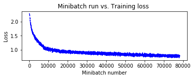
◆ 前節のモデル定義は非常に単純ですが、C.layers.For を利用すれば更に簡潔になります。
この程度のモデルであれば無理に C.layers.For を使用することもありませんが、より深層なモデルになれば有用でしょう :
def create_basic_model_terse(input, out_dims):

    with C.layers.default_options(init=C.glorot_uniform(), activation=C.relu):
        model = C.layers.Sequential([
            C.layers.For(range(3), lambda i: [
                C.layers.Convolution((5,5), [32,32,64][i], pad=True),
                C.layers.MaxPooling((3,3), strides=(2,2))
                ]),
            C.layers.Dense(64),
            C.layers.Dense(out_dims, activation=None)
        ])

    return model(input)
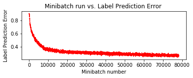
もちろん同様の結果にしかなりませんが、念のために 100 エポック訓練してみましょう :
%%time
pred_basic_model = train_and_evaluate(reader_train,
                                      reader_test,
                                      max_epochs=100,
                                      model_func=create_basic_model_terse)
Training 116906 parameters in 10 parameter tensors.

Learning rate per minibatch: 0.01
Momentum per 1 samples: 0.9983550962823424
Finished Epoch[1 of 100]: [Training] loss = 2.107097 * 50000, metric = 78.58% * 50000 7.111s (7031.4 samples/s);
Finished Epoch[2 of 100]: [Training] loss = 1.752438 * 50000, metric = 64.54% * 50000 6.974s (7169.5 samples/s);
Finished Epoch[3 of 100]: [Training] loss = 1.576601 * 50000, metric = 57.93% * 50000 6.799s (7354.0 samples/s);
Finished Epoch[4 of 100]: [Training] loss = 1.472111 * 50000, metric = 53.73% * 50000 6.693s (7470.5 samples/s);
Finished Epoch[5 of 100]: [Training] loss = 1.385220 * 50000, metric = 50.05% * 50000 6.871s (7277.0 samples/s);
Finished Epoch[6 of 100]: [Training] loss = 1.316881 * 50000, metric = 47.20% * 50000 6.915s (7230.7 samples/s);
Finished Epoch[7 of 100]: [Training] loss = 1.243615 * 50000, metric = 44.27% * 50000 6.847s (7302.5 samples/s);
Finished Epoch[8 of 100]: [Training] loss = 1.193445 * 50000, metric = 42.24% * 50000 6.772s (7383.3 samples/s);
Finished Epoch[9 of 100]: [Training] loss = 1.142968 * 50000, metric = 40.29% * 50000 6.914s (7231.7 samples/s);
Finished Epoch[10 of 100]: [Training] loss = 1.101501 * 50000, metric = 38.83% * 50000 6.771s (7384.4 samples/s);
Learning rate per minibatch: 0.003
Finished Epoch[11 of 100]: [Training] loss = 1.044963 * 50000, metric = 36.69% * 50000 6.759s (7397.5 samples/s);
Finished Epoch[12 of 100]: [Training] loss = 1.026290 * 50000, metric = 35.95% * 50000 6.931s (7214.0 samples/s);
Finished Epoch[13 of 100]: [Training] loss = 1.018971 * 50000, metric = 35.86% * 50000 6.894s (7252.7 samples/s);
Finished Epoch[14 of 100]: [Training] loss = 1.005527 * 50000, metric = 35.29% * 50000 6.706s (7456.0 samples/s);
Finished Epoch[15 of 100]: [Training] loss = 0.994635 * 50000, metric = 34.74% * 50000 6.761s (7395.4 samples/s);
Finished Epoch[16 of 100]: [Training] loss = 0.987681 * 50000, metric = 34.59% * 50000 6.964s (7179.8 samples/s);
Finished Epoch[17 of 100]: [Training] loss = 0.978682 * 50000, metric = 34.13% * 50000 6.855s (7293.9 samples/s);
Finished Epoch[18 of 100]: [Training] loss = 0.967565 * 50000, metric = 33.94% * 50000 6.812s (7340.0 samples/s);
Finished Epoch[19 of 100]: [Training] loss = 0.959276 * 50000, metric = 33.54% * 50000 6.717s (7443.8 samples/s);
Finished Epoch[20 of 100]: [Training] loss = 0.952435 * 50000, metric = 33.38% * 50000 6.856s (7292.9 samples/s);
Learning rate per minibatch: 0.001
Finished Epoch[21 of 100]: [Training] loss = 0.928293 * 50000, metric = 32.27% * 50000 6.805s (7347.5 samples/s);
Finished Epoch[22 of 100]: [Training] loss = 0.930338 * 50000, metric = 32.33% * 50000 6.857s (7291.8 samples/s);
Finished Epoch[23 of 100]: [Training] loss = 0.928376 * 50000, metric = 32.29% * 50000 6.911s (7234.8 samples/s);
Finished Epoch[24 of 100]: [Training] loss = 0.921075 * 50000, metric = 32.10% * 50000 6.885s (7262.2 samples/s);
Finished Epoch[25 of 100]: [Training] loss = 0.921620 * 50000, metric = 32.20% * 50000 6.931s (7214.0 samples/s);
Finished Epoch[26 of 100]: [Training] loss = 0.915684 * 50000, metric = 31.80% * 50000 6.950s (7194.2 samples/s);
Finished Epoch[27 of 100]: [Training] loss = 0.916585 * 50000, metric = 31.79% * 50000 6.783s (7371.4 samples/s);
Finished Epoch[28 of 100]: [Training] loss = 0.910325 * 50000, metric = 31.68% * 50000 6.847s (7302.5 samples/s);
Finished Epoch[29 of 100]: [Training] loss = 0.905840 * 50000, metric = 31.42% * 50000 6.771s (7384.4 samples/s);
Finished Epoch[30 of 100]: [Training] loss = 0.908549 * 50000, metric = 31.65% * 50000 6.815s (7336.8 samples/s);

Finished Epoch[40 of 100]: [Training] loss = 0.877802 * 50000, metric = 30.34% * 50000 6.784s (7370.3 samples/s);

Finished Epoch[50 of 100]: [Training] loss = 0.860325 * 50000, metric = 29.95% * 50000 6.731s (7428.3 samples/s);

Finished Epoch[60 of 100]: [Training] loss = 0.838169 * 50000, metric = 29.01% * 50000 6.862s (7286.5 samples/s);

Finished Epoch[70 of 100]: [Training] loss = 0.814805 * 50000, metric = 28.40% * 50000 6.775s (7380.1 samples/s);

Finished Epoch[80 of 100]: [Training] loss = 0.800001 * 50000, metric = 27.63% * 50000 6.853s (7296.1 samples/s);

Finished Epoch[90 of 100]: [Training] loss = 0.779285 * 50000, metric = 27.10% * 50000 6.892s (7254.8 samples/s);

Finished Epoch[100 of 100]: [Training] loss = 0.759459 * 50000, metric = 26.39% * 50000 7.079s (7063.1 samples/s);

Final Results: Minibatch[1-626]: errs = 25.5% * 10000
CPU times: user 15min 12s, sys: 2min 11s, total: 17min 24s
Wall time: 9min 3s
訓練されたモデルを得ましたので、次のトラックの画像を分類してみます。画像を読むためには PIL ライブラリを使用します :
Image(url="https://cntk.ai/jup/201/00014.png", width=64, height=64)

# サンプル画像をダウンロードします (これはテスト・データセットの 00014.png です)。
# サイズ 32, 32 の任意の画像が評価できます。
url = "https://cntk.ai/jup/201/00014.png"
myimg = np.array(PIL.Image.open(urlopen(url)), dtype=np.float32)
訓練の間、入力画像から平均を減算していましたので、ここでも平均の近似値を用いて画像から減算します :
def eval(pred_op, image_data):
    label_lookup = ["airplane", "automobile", "bird", "cat", "deer", "dog", "frog", "horse", "ship", "truck"]
    image_mean = 133.0
    image_data -= image_mean
    image_data = np.ascontiguousarray(np.transpose(image_data, (2, 0, 1)))

    result = np.squeeze(pred_op.eval({pred_op.arguments[0]:[image_data]}))

    # Return top 3 results:
    top_count = 3
    result_indices = (-np.array(result)).argsort()[:top_count]

    print("Top 3 predictions:")
    for i in range(top_count):
        print("\tLabel: {:10s}, confidence: {:.2f}%".format(label_lookup[result_indices[i]], result[result_indices[i]] * 100))
# Run the evaluation on the downloaded image
eval(pred_basic_model, myimg)
Top 3 predictions:
	Label: truck     , confidence: 95.28%
	Label: ship      , confidence: 4.22%
	Label: automobile, confidence: 0.40%
※ ここで GPU メモリを確認しておきます。
$ nvidia-smi
Sun Oct 29 15:44:15 2017
+-----------------------------------------------------------------------------+
| NVIDIA-SMI 384.90                 Driver Version: 384.90                    |
|-------------------------------+----------------------+----------------------+
| GPU  Name        Persistence-M| Bus-Id        Disp.A | Volatile Uncorr. ECC |
| Fan  Temp  Perf  Pwr:Usage/Cap|         Memory-Usage | GPU-Util  Compute M. |
|===============================+======================+======================|
|   0  Tesla K80           Off  | 0000F196:00:00.0 Off |                    0 |
| N/A   58C    P0    56W / 149W |    298MiB / 11439MiB |      0%      Default |
+-------------------------------+----------------------+----------------------+

+-----------------------------------------------------------------------------+
| Processes:                                                       GPU Memory |
|  GPU       PID   Type   Process name                             Usage      |
|=============================================================================|
|    0     11732      C   /home/masao/anaconda3/bin/python             285MiB |
+-----------------------------------------------------------------------------+
4-6 ドロップアウト層を持つ CNN モデル
ドロップアウト層を追加してみましょう。
最後の Dense 層の前にドロップ率 0.25 でドロップ層を追加します :
def create_basic_model_with_dropout(input, out_dims):

    with C.layers.default_options(activation=C.relu, init=C.glorot_uniform()):
        model = C.layers.Sequential([
            C.layers.For(range(3), lambda i: [
                C.layers.Convolution((5,5), [32,32,64][i], pad=True),
                C.layers.MaxPooling((3,3), strides=(2,2))
            ]),
            C.layers.Dense(64),
            C.layers.Dropout(0.25),
            C.layers.Dense(out_dims, activation=None)
        ])

    return model(input)
ドロップアウト層の追加はオーバーフィッティングの回避に有効ですが、同じ精度を得るために訓練時間はより多くかかります。
ここでは 150 エポック訓練しましょう :
%%time
pred_basic_model_dropout = train_and_evaluate(reader_train,
                                              reader_test,
                                              max_epochs=150,
                                              model_func=create_basic_model_with_dropout)
Training 116906 parameters in 10 parameter tensors.

Learning rate per minibatch: 0.01
Momentum per 1 samples: 0.9983550962823424
Finished Epoch[1 of 150]: [Training] loss = 2.107362 * 50000, metric = 78.56% * 50000 7.048s (7094.2 samples/s);
Finished Epoch[2 of 150]: [Training] loss = 1.795894 * 50000, metric = 66.94% * 50000 6.775s (7380.1 samples/s);
Finished Epoch[3 of 150]: [Training] loss = 1.653298 * 50000, metric = 61.18% * 50000 6.885s (7262.2 samples/s);
Finished Epoch[4 of 150]: [Training] loss = 1.561897 * 50000, metric = 57.29% * 50000 6.997s (7145.9 samples/s);
Finished Epoch[5 of 150]: [Training] loss = 1.488496 * 50000, metric = 54.18% * 50000 6.817s (7334.6 samples/s);
Finished Epoch[6 of 150]: [Training] loss = 1.424205 * 50000, metric = 51.39% * 50000 6.940s (7204.6 samples/s);
Finished Epoch[7 of 150]: [Training] loss = 1.368698 * 50000, metric = 49.17% * 50000 6.821s (7330.3 samples/s);
Finished Epoch[8 of 150]: [Training] loss = 1.314402 * 50000, metric = 46.99% * 50000 6.956s (7188.0 samples/s);
Finished Epoch[9 of 150]: [Training] loss = 1.263993 * 50000, metric = 45.21% * 50000 6.937s (7207.7 samples/s);
Finished Epoch[10 of 150]: [Training] loss = 1.219663 * 50000, metric = 43.65% * 50000 6.957s (7187.0 samples/s);
Learning rate per minibatch: 0.003
Finished Epoch[11 of 150]: [Training] loss = 1.163245 * 50000, metric = 41.54% * 50000 6.794s (7359.4 samples/s);
Finished Epoch[12 of 150]: [Training] loss = 1.147450 * 50000, metric = 40.75% * 50000 6.847s (7302.5 samples/s);
Finished Epoch[13 of 150]: [Training] loss = 1.133124 * 50000, metric = 40.20% * 50000 6.797s (7356.2 samples/s);
Finished Epoch[14 of 150]: [Training] loss = 1.123846 * 50000, metric = 39.65% * 50000 6.874s (7273.8 samples/s);
Finished Epoch[15 of 150]: [Training] loss = 1.113345 * 50000, metric = 39.39% * 50000 6.972s (7171.5 samples/s);
Finished Epoch[16 of 150]: [Training] loss = 1.103626 * 50000, metric = 39.06% * 50000 6.832s (7318.5 samples/s);
Finished Epoch[17 of 150]: [Training] loss = 1.092183 * 50000, metric = 38.46% * 50000 6.973s (7170.5 samples/s);
Finished Epoch[18 of 150]: [Training] loss = 1.085112 * 50000, metric = 38.40% * 50000 7.011s (7131.7 samples/s);
Finished Epoch[19 of 150]: [Training] loss = 1.076314 * 50000, metric = 37.92% * 50000 6.810s (7342.1 samples/s);
Finished Epoch[20 of 150]: [Training] loss = 1.069802 * 50000, metric = 37.85% * 50000 7.018s (7124.5 samples/s);
Learning rate per minibatch: 0.001
Finished Epoch[21 of 150]: [Training] loss = 1.049303 * 50000, metric = 37.02% * 50000 6.920s (7225.4 samples/s);
Finished Epoch[22 of 150]: [Training] loss = 1.043940 * 50000, metric = 36.70% * 50000 6.890s (7256.9 samples/s);
Finished Epoch[23 of 150]: [Training] loss = 1.038793 * 50000, metric = 36.66% * 50000 6.965s (7178.8 samples/s);
Finished Epoch[24 of 150]: [Training] loss = 1.036304 * 50000, metric = 36.60% * 50000 6.651s (7517.7 samples/s);
Finished Epoch[25 of 150]: [Training] loss = 1.028823 * 50000, metric = 36.24% * 50000 6.837s (7313.1 samples/s);
Finished Epoch[26 of 150]: [Training] loss = 1.029764 * 50000, metric = 36.17% * 50000 6.876s (7271.7 samples/s);
Finished Epoch[27 of 150]: [Training] loss = 1.028118 * 50000, metric = 36.03% * 50000 6.929s (7216.0 samples/s);
Finished Epoch[28 of 150]: [Training] loss = 1.027320 * 50000, metric = 36.19% * 50000 6.901s (7245.3 samples/s);
Finished Epoch[29 of 150]: [Training] loss = 1.023353 * 50000, metric = 35.82% * 50000 6.925s (7220.2 samples/s);
Finished Epoch[30 of 150]: [Training] loss = 1.023630 * 50000, metric = 35.89% * 50000 6.981s (7162.3 samples/s);

Finished Epoch[40 of 150]: [Training] loss = 0.993943 * 50000, metric = 34.95% * 50000 7.010s (7132.7 samples/s);

Finished Epoch[50 of 150]: [Training] loss = 0.965364 * 50000, metric = 33.83% * 50000 6.786s (7368.1 samples/s);

Finished Epoch[60 of 150]: [Training] loss = 0.947730 * 50000, metric = 33.10% * 50000 6.838s (7312.1 samples/s);

Finished Epoch[70 of 150]: [Training] loss = 0.927696 * 50000, metric = 32.38% * 50000 6.827s (7323.9 samples/s);

Finished Epoch[80 of 150]: [Training] loss = 0.906988 * 50000, metric = 31.91% * 50000 6.939s (7205.6 samples/s);

Finished Epoch[90 of 150]: [Training] loss = 0.891659 * 50000, metric = 30.84% * 50000 6.918s (7227.5 samples/s);

Finished Epoch[100 of 150]: [Training] loss = 0.875521 * 50000, metric = 30.51% * 50000 6.675s (7490.6 samples/s);

Finished Epoch[110 of 150]: [Training] loss = 0.850758 * 50000, metric = 29.29% * 50000 6.982s (7161.3 samples/s);

Finished Epoch[120 of 150]: [Training] loss = 0.841164 * 50000, metric = 29.22% * 50000 6.996s (7146.9 samples/s);

Finished Epoch[130 of 150]: [Training] loss = 0.828868 * 50000, metric = 28.51% * 50000 7.002s (7140.8 samples/s);

Finished Epoch[140 of 150]: [Training] loss = 0.818199 * 50000, metric = 28.17% * 50000 6.912s (7233.8 samples/s);

Finished Epoch[150 of 150]: [Training] loss = 0.801844 * 50000, metric = 27.54% * 50000 6.879s (7268.5 samples/s);

Final Results: Minibatch[1-626]: errs = 25.5% * 10000
CPU times: user 22min 26s, sys: 2min 57s, total: 25min 24s
Wall time: 12min 38s
$ nvidia-smi
Sun Oct 29 16:00:59 2017
+-----------------------------------------------------------------------------+
| NVIDIA-SMI 384.90                 Driver Version: 384.90                    |
|-------------------------------+----------------------+----------------------+
| GPU  Name        Persistence-M| Bus-Id        Disp.A | Volatile Uncorr. ECC |
| Fan  Temp  Perf  Pwr:Usage/Cap|         Memory-Usage | GPU-Util  Compute M. |
|===============================+======================+======================|
|   0  Tesla K80           Off  | 0000F196:00:00.0 Off |                    0 |
| N/A   59C    P0    56W / 149W |    300MiB / 11439MiB |      0%      Default |
+-------------------------------+----------------------+----------------------+

+-----------------------------------------------------------------------------+
| Processes:                                                       GPU Memory |
|  GPU       PID   Type   Process name                             Usage      |
|=============================================================================|
|    0     11732      C   /home/masao/anaconda3/bin/python             287MiB |
+-----------------------------------------------------------------------------+
4-7 BN 層を持つ CNN モデル
基本モデルの改良の最後に、バッチ正規化層を追加します。これは精度を劇的に上げてくれます。
追加する位置は各畳み込み層の後と最後の Dense 層の前です :
def create_basic_model_with_batch_normalization(input, out_dims):

    with C.layers.default_options(activation=C.relu, init=C.glorot_uniform()):
        model = C.layers.Sequential([
            C.layers.For(range(3), lambda i: [
                C.layers.Convolution((5,5), [32,32,64][i], pad=True),
                C.layers.BatchNormalization(map_rank=1),
                C.layers.MaxPooling((3,3), strides=(2,2))
            ]),
            C.layers.Dense(64),
            C.layers.BatchNormalization(map_rank=1),
            C.layers.Dense(out_dims, activation=None)
        ])

    return model(input)
%%time
pred_basic_model_bn = train_and_evaluate(reader_train,
                                         reader_test,
                                         max_epochs=150,
                                         model_func=create_basic_model_with_batch_normalization)
Training 117290 parameters in 18 parameter tensors.

Learning rate per minibatch: 0.01
Momentum per 1 samples: 0.9983550962823424
Finished Epoch[1 of 150]: [Training] loss = 1.575825 * 50000, metric = 56.10% * 50000 8.114s (6162.2 samples/s);
Finished Epoch[2 of 150]: [Training] loss = 1.214922 * 50000, metric = 43.03% * 50000 7.782s (6425.1 samples/s);
Finished Epoch[3 of 150]: [Training] loss = 1.074148 * 50000, metric = 37.63% * 50000 7.818s (6395.5 samples/s);
Finished Epoch[4 of 150]: [Training] loss = 0.998258 * 50000, metric = 34.84% * 50000 7.895s (6333.1 samples/s);
Finished Epoch[5 of 150]: [Training] loss = 0.940484 * 50000, metric = 32.72% * 50000 7.719s (6477.5 samples/s);
Finished Epoch[6 of 150]: [Training] loss = 0.896672 * 50000, metric = 31.30% * 50000 7.822s (6392.2 samples/s);
Finished Epoch[7 of 150]: [Training] loss = 0.861366 * 50000, metric = 30.15% * 50000 7.879s (6346.0 samples/s);
Finished Epoch[8 of 150]: [Training] loss = 0.831189 * 50000, metric = 28.80% * 50000 7.847s (6371.9 samples/s);
Finished Epoch[9 of 150]: [Training] loss = 0.804354 * 50000, metric = 28.19% * 50000 7.975s (6269.6 samples/s);
Finished Epoch[10 of 150]: [Training] loss = 0.780050 * 50000, metric = 27.10% * 50000 7.717s (6479.2 samples/s);
Learning rate per minibatch: 0.003
Finished Epoch[11 of 150]: [Training] loss = 0.730435 * 50000, metric = 25.12% * 50000 7.870s (6353.2 samples/s);
Finished Epoch[12 of 150]: [Training] loss = 0.719849 * 50000, metric = 25.01% * 50000 7.722s (6475.0 samples/s);
Finished Epoch[13 of 150]: [Training] loss = 0.705523 * 50000, metric = 24.43% * 50000 7.939s (6298.0 samples/s);
Finished Epoch[14 of 150]: [Training] loss = 0.704748 * 50000, metric = 24.24% * 50000 7.752s (6449.9 samples/s);
Finished Epoch[15 of 150]: [Training] loss = 0.692881 * 50000, metric = 24.04% * 50000 7.881s (6344.4 samples/s);
Finished Epoch[16 of 150]: [Training] loss = 0.689439 * 50000, metric = 23.68% * 50000 7.840s (6377.6 samples/s);
Finished Epoch[17 of 150]: [Training] loss = 0.685853 * 50000, metric = 23.75% * 50000 7.874s (6350.0 samples/s);
Finished Epoch[18 of 150]: [Training] loss = 0.682089 * 50000, metric = 23.48% * 50000 7.810s (6402.0 samples/s);
Finished Epoch[19 of 150]: [Training] loss = 0.673679 * 50000, metric = 23.18% * 50000 7.818s (6395.5 samples/s);
Finished Epoch[20 of 150]: [Training] loss = 0.679083 * 50000, metric = 23.39% * 50000 7.829s (6386.5 samples/s);
Learning rate per minibatch: 0.001
Finished Epoch[21 of 150]: [Training] loss = 0.652570 * 50000, metric = 22.71% * 50000 7.769s (6435.8 samples/s);
Finished Epoch[22 of 150]: [Training] loss = 0.646894 * 50000, metric = 22.45% * 50000 7.836s (6380.8 samples/s);
Finished Epoch[23 of 150]: [Training] loss = 0.649195 * 50000, metric = 22.50% * 50000 7.855s (6365.4 samples/s);
Finished Epoch[24 of 150]: [Training] loss = 0.642438 * 50000, metric = 22.12% * 50000 7.789s (6419.3 samples/s);
Finished Epoch[25 of 150]: [Training] loss = 0.647353 * 50000, metric = 22.47% * 50000 7.776s (6430.0 samples/s);
Finished Epoch[26 of 150]: [Training] loss = 0.637380 * 50000, metric = 22.17% * 50000 7.683s (6507.9 samples/s);
Finished Epoch[27 of 150]: [Training] loss = 0.637883 * 50000, metric = 22.02% * 50000 7.694s (6498.6 samples/s);
Finished Epoch[28 of 150]: [Training] loss = 0.632257 * 50000, metric = 21.96% * 50000 7.726s (6471.7 samples/s);
Finished Epoch[29 of 150]: [Training] loss = 0.631863 * 50000, metric = 21.76% * 50000 7.762s (6441.6 samples/s);
Finished Epoch[30 of 150]: [Training] loss = 0.631520 * 50000, metric = 21.84% * 50000 7.691s (6501.1 samples/s);

Finished Epoch[40 of 150]: [Training] loss = 0.617032 * 50000, metric = 21.28% * 50000 7.775s (6430.9 samples/s);

Finished Epoch[50 of 150]: [Training] loss = 0.598427 * 50000, metric = 20.46% * 50000 7.723s (6474.2 samples/s);

Finished Epoch[60 of 150]: [Training] loss = 0.584324 * 50000, metric = 20.14% * 50000 7.868s (6354.9 samples/s);

Finished Epoch[70 of 150]: [Training] loss = 0.571565 * 50000, metric = 19.51% * 50000 7.983s (6263.3 samples/s);

Finished Epoch[80 of 150]: [Training] loss = 0.559020 * 50000, metric = 19.18% * 50000 7.910s (6321.1 samples/s);

Finished Epoch[90 of 150]: [Training] loss = 0.549592 * 50000, metric = 19.10% * 50000 7.735s (6464.1 samples/s);

Finished Epoch[100 of 150]: [Training] loss = 0.540868 * 50000, metric = 18.79% * 50000 7.715s (6480.9 samples/s);

Finished Epoch[110 of 150]: [Training] loss = 0.527440 * 50000, metric = 18.28% * 50000 7.703s (6491.0 samples/s);

Finished Epoch[120 of 150]: [Training] loss = 0.518411 * 50000, metric = 17.94% * 50000 7.903s (6326.7 samples/s);

Finished Epoch[130 of 150]: [Training] loss = 0.509930 * 50000, metric = 17.77% * 50000 7.711s (6484.2 samples/s);

Finished Epoch[140 of 150]: [Training] loss = 0.499302 * 50000, metric = 17.38% * 50000 7.880s (6345.2 samples/s);

Finished Epoch[150 of 150]: [Training] loss = 0.497221 * 50000, metric = 17.26% * 50000 7.807s (6404.5 samples/s);

Final Results: Minibatch[1-626]: errs = 17.9% * 10000
CPU times: user 25min 2s, sys: 3min 38s, total: 28min 40s
Wall time: 15min 48s
テスト精度が 80 % を超え、82.1 % を得ました!
$ nvidia-smi
Sun Oct 29 16:22:42 2017
+-----------------------------------------------------------------------------+
| NVIDIA-SMI 384.90                 Driver Version: 384.90                    |
|-------------------------------+----------------------+----------------------+
| GPU  Name        Persistence-M| Bus-Id        Disp.A | Volatile Uncorr. ECC |
| Fan  Temp  Perf  Pwr:Usage/Cap|         Memory-Usage | GPU-Util  Compute M. |
|===============================+======================+======================|
|   0  Tesla K80           Off  | 0000F196:00:00.0 Off |                    0 |
| N/A   57C    P0    56W / 149W |    300MiB / 11439MiB |      0%      Default |
+-------------------------------+----------------------+----------------------+

+-----------------------------------------------------------------------------+
| Processes:                                                       GPU Memory |
|  GPU       PID   Type   Process name                             Usage      |
|=============================================================================|
|    0     11732      C   /home/masao/anaconda3/bin/python             287MiB |
+-----------------------------------------------------------------------------+
5.VGG
基本モデルにバッチ正規化層を追加する改良でテスト精度 80 % 超えを果たしましたが、ここから先はモデルの見直しが必要になります。
そこで次に VGG を CNTK で実装してみます。VGG を特徴づけるのは以下のようなポイントです :
- 総ての畳み込み層は 3 x 3 の畳み込みカーネルを持ちます。
- 畳み込み層を 2 層以上積層したブロックを複数個スタックします。
- ブロックの区切りはマックス・プーリングです。
- 通常は BN 層は持ちません。
本来の VGG-19 や VGG-16 モデルをそのまま CIFAR-10 に適用すると特徴マップが小さくなり過ぎますので、
ブロック数を減らして簡略化した VGG-9 なるものを考えて実装します。
※ VGG- の後の数字は畳み込み層と Dense 層の総数です。
※ VGG-9 は正式な用語ではありません、念のため。
VGG-9 のアーキテクチャは以下の図のようなものです :
| VGG-9 |
|---|
| conv3-64 |
| conv3-64 |
| max3 |
| conv3-96 |
| conv3-96 |
| max3 |
| conv3-128 |
| conv3-128 |
| max3 |
| FC-1024 |
| FC-1024 |
| FC-10 |
CNTK で簡単に実装できます :
def create_vgg9_model(input, out_dims):
    with C.layers.default_options(activation=C.relu, init=C.glorot_uniform()):
        model = C.layers.Sequential([
            C.layers.For(range(3), lambda i: [
                C.layers.Convolution((3,3), [64,96,128][i], pad=True),
                C.layers.Convolution((3,3), [64,96,128][i], pad=True),
                C.layers.MaxPooling((3,3), strides=(2,2))
            ]),
            C.layers.For(range(2), lambda : [
                C.layers.Dense(1024)
            ]),
            C.layers.Dense(out_dims, activation=None)
        ])

    return model(input)
少し多めに 200 エポック訓練してみましょう :
%%time
pred_vgg = train_and_evaluate(reader_train,
                              reader_test,
                              max_epochs=200,
                              model_func=create_vgg9_model)
Training 2675978 parameters in 18 parameter tensors.

Learning rate per minibatch: 0.01
Momentum per 1 samples: 0.9983550962823424
Finished Epoch[1 of 200]: [Training] loss = 2.285345 * 50000, metric = 85.05% * 50000 21.439s (2332.2 samples/s);
Finished Epoch[2 of 200]: [Training] loss = 1.950674 * 50000, metric = 72.51% * 50000 20.717s (2413.5 samples/s);
Finished Epoch[3 of 200]: [Training] loss = 1.703872 * 50000, metric = 63.54% * 50000 20.750s (2409.6 samples/s);
Finished Epoch[4 of 200]: [Training] loss = 1.569704 * 50000, metric = 57.85% * 50000 20.852s (2397.9 samples/s);
Finished Epoch[5 of 200]: [Training] loss = 1.470902 * 50000, metric = 53.46% * 50000 20.808s (2402.9 samples/s);
Finished Epoch[6 of 200]: [Training] loss = 1.386016 * 50000, metric = 49.94% * 50000 20.818s (2401.8 samples/s);
Finished Epoch[7 of 200]: [Training] loss = 1.303779 * 50000, metric = 46.89% * 50000 20.857s (2397.3 samples/s);
Finished Epoch[8 of 200]: [Training] loss = 1.228470 * 50000, metric = 44.09% * 50000 20.777s (2406.5 samples/s);
Finished Epoch[9 of 200]: [Training] loss = 1.164719 * 50000, metric = 41.57% * 50000 20.754s (2409.2 samples/s);
Finished Epoch[10 of 200]: [Training] loss = 1.082482 * 50000, metric = 38.66% * 50000 20.830s (2400.4 samples/s);
Learning rate per minibatch: 0.003
Finished Epoch[11 of 200]: [Training] loss = 0.995793 * 50000, metric = 35.41% * 50000 20.787s (2405.3 samples/s);
Finished Epoch[12 of 200]: [Training] loss = 0.973461 * 50000, metric = 34.58% * 50000 20.787s (2405.3 samples/s);
Finished Epoch[13 of 200]: [Training] loss = 0.954539 * 50000, metric = 33.78% * 50000 20.834s (2399.9 samples/s);
Finished Epoch[14 of 200]: [Training] loss = 0.932364 * 50000, metric = 32.92% * 50000 20.795s (2404.4 samples/s);
Finished Epoch[15 of 200]: [Training] loss = 0.918446 * 50000, metric = 32.77% * 50000 20.784s (2405.7 samples/s);
Finished Epoch[16 of 200]: [Training] loss = 0.898028 * 50000, metric = 31.81% * 50000 20.802s (2403.6 samples/s);
Finished Epoch[17 of 200]: [Training] loss = 0.880874 * 50000, metric = 31.10% * 50000 20.784s (2405.7 samples/s);
Finished Epoch[18 of 200]: [Training] loss = 0.871529 * 50000, metric = 30.57% * 50000 20.741s (2410.7 samples/s);
Finished Epoch[19 of 200]: [Training] loss = 0.857613 * 50000, metric = 30.20% * 50000 20.845s (2398.7 samples/s);
Finished Epoch[20 of 200]: [Training] loss = 0.848898 * 50000, metric = 29.92% * 50000 20.822s (2401.3 samples/s);
Learning rate per minibatch: 0.001
Finished Epoch[21 of 200]: [Training] loss = 0.805457 * 50000, metric = 28.39% * 50000 20.791s (2404.9 samples/s);
Finished Epoch[22 of 200]: [Training] loss = 0.800717 * 50000, metric = 28.19% * 50000 20.801s (2403.7 samples/s);
Finished Epoch[23 of 200]: [Training] loss = 0.793407 * 50000, metric = 27.89% * 50000 20.797s (2404.2 samples/s);
Finished Epoch[24 of 200]: [Training] loss = 0.788432 * 50000, metric = 27.92% * 50000 20.806s (2403.2 samples/s);
Finished Epoch[25 of 200]: [Training] loss = 0.783144 * 50000, metric = 27.25% * 50000 20.744s (2410.3 samples/s);
Finished Epoch[26 of 200]: [Training] loss = 0.783097 * 50000, metric = 27.37% * 50000 20.814s (2402.2 samples/s);
Finished Epoch[27 of 200]: [Training] loss = 0.775362 * 50000, metric = 27.14% * 50000 20.841s (2399.1 samples/s);
Finished Epoch[28 of 200]: [Training] loss = 0.764829 * 50000, metric = 26.73% * 50000 20.869s (2395.9 samples/s);
Finished Epoch[29 of 200]: [Training] loss = 0.765971 * 50000, metric = 26.76% * 50000 20.743s (2410.5 samples/s);
Finished Epoch[30 of 200]: [Training] loss = 0.760259 * 50000, metric = 26.39% * 50000 20.758s (2408.7 samples/s);

Finished Epoch[40 of 200]: [Training] loss = 0.723249 * 50000, metric = 25.29% * 50000 20.811s (2402.6 samples/s);

Finished Epoch[50 of 200]: [Training] loss = 0.690826 * 50000, metric = 24.10% * 50000 20.792s (2404.8 samples/s);

Finished Epoch[60 of 200]: [Training] loss = 0.661614 * 50000, metric = 23.08% * 50000 20.844s (2398.8 samples/s);

Finished Epoch[70 of 200]: [Training] loss = 0.640153 * 50000, metric = 22.53% * 50000 20.819s (2401.7 samples/s);

Finished Epoch[80 of 200]: [Training] loss = 0.616333 * 50000, metric = 21.58% * 50000 20.774s (2406.9 samples/s);

Finished Epoch[90 of 200]: [Training] loss = 0.590828 * 50000, metric = 20.66% * 50000 20.801s (2403.7 samples/s);

Finished Epoch[100 of 200]: [Training] loss = 0.573662 * 50000, metric = 19.89% * 50000 20.862s (2396.7 samples/s);

Finished Epoch[110 of 200]: [Training] loss = 0.554091 * 50000, metric = 19.32% * 50000 20.791s (2404.9 samples/s);

Finished Epoch[120 of 200]: [Training] loss = 0.541163 * 50000, metric = 18.96% * 50000 20.863s (2396.6 samples/s);

Finished Epoch[130 of 200]: [Training] loss = 0.518876 * 50000, metric = 18.21% * 50000 20.821s (2401.4 samples/s);

Finished Epoch[140 of 200]: [Training] loss = 0.512452 * 50000, metric = 17.87% * 50000 20.816s (2402.0 samples/s);

Finished Epoch[150 of 200]: [Training] loss = 0.493485 * 50000, metric = 17.41% * 50000 20.836s (2399.7 samples/s);

Finished Epoch[160 of 200]: [Training] loss = 0.483110 * 50000, metric = 16.83% * 50000 20.808s (2402.9 samples/s);

Finished Epoch[170 of 200]: [Training] loss = 0.467576 * 50000, metric = 16.43% * 50000 20.822s (2401.3 samples/s);

Finished Epoch[180 of 200]: [Training] loss = 0.452476 * 50000, metric = 15.75% * 50000 20.855s (2397.5 samples/s);

Finished Epoch[190 of 200]: [Training] loss = 0.438725 * 50000, metric = 15.30% * 50000 20.781s (2406.0 samples/s);

Finished Epoch[200 of 200]: [Training] loss = 0.430123 * 50000, metric = 15.01% * 50000 20.819s (2401.7 samples/s);

Final Results: Minibatch[1-626]: errs = 16.7% * 10000
CPU times: user 1h 11min 54s, sys: 11min 59s, total: 1h 23min 53s
Wall time: 1h 6min 21s
テスト精度 83.3 % が得られました!
$ nvidia-smi
Sun Oct 29 17:30:50 2017
+-----------------------------------------------------------------------------+
| NVIDIA-SMI 384.90                 Driver Version: 384.90                    |
|-------------------------------+----------------------+----------------------+
| GPU  Name        Persistence-M| Bus-Id        Disp.A | Volatile Uncorr. ECC |
| Fan  Temp  Perf  Pwr:Usage/Cap|         Memory-Usage | GPU-Util  Compute M. |
|===============================+======================+======================|
|   0  Tesla K80           Off  | 0000F196:00:00.0 Off |                    0 |
| N/A   66C    P0    57W / 149W |    312MiB / 11439MiB |      0%      Default |
+-------------------------------+----------------------+----------------------+

+-----------------------------------------------------------------------------+
| Processes:                                                       GPU Memory |
|  GPU       PID   Type   Process name                             Usage      |
|=============================================================================|
|    0     11732      C   /home/masao/anaconda3/bin/python             299MiB |
+-----------------------------------------------------------------------------+
6. Residual Network (ResNet)
VGG は層を深くすることによって学習能力を高めていきましたが、20 層以上に層を単純に深くしても上手く学習は進みません。
層が深くなると勾配消失したり発散するという基本的な問題に加えて、(層数が少ないモデルに比較して) 精度が逆に悪くなるという現象も見られます。そのために様々なアプローチが工夫されています。
ResNet ( Deep Residual Learning for Image Recognition ) はそのような degradation (劣化) 問題に対処するために、MSRA の研究者により考案されたモデルで、152 層まで深くなっています。派生したモデルも数多く重要な位置づけにあります。
ResNet は残差の話しが直感的に分かりにくいのですが、アーキテクチャ - Deep Residual Learning Framework のビルディング・ブロックは単純です。
(下図のような) 恒等マッピングの機能を有するショートカット接続を持つような (畳み込み層の) 積層ブロックのスタックで構成される、ショートカット接続つきの順伝播ニューラルネットワークとして ResNet は定義されます :
Image(url="https://cntk.ai/jup/201/ResNetBlock2.png")

要するに、ブロックへの入力を参照させます。ブロックの出口の活性化関数への入力として、ブロックの入口の入力を加算します。これがショートカットです。このショートカットが恒等マッピングとしての機能を果たし、これが層が深くなった時に良い作用をします (ショートカットがない場合よりも学習が進みやすくなります)。
層が深くなったときには、ブロックは恒等マッピングに限りなく近いはず、という発想です。本来のパスの積層の重みがゼロになればブロックは恒等関数になります。
実装するためにはこれだけの情報で十分です。
なお、上図の左側が plain なブロックで、右側はボトルネックと呼ばれます。
今回はボトルネックは使いませんが、より深くなっているので良い結果が得られるようです。
本記事は CNTK による実装が目的ですので、理論的な側面については深入りしませんが、
概要を知りたいのであれば以下のスライドを参考にすると良いでしょう :
また、ResNet の解釈としては (私見ですが) 以下は良いヒントを与えてくれます。パスの長さに着目してネットワークを展開して考察しています :
Residual Networks Behave Like Ensembles of Relatively Shallow Networks
◆ さて、CNTK を使用して以下の ResNet ブロックを実装してみましょう。意外に簡単です :
            ResNetNode                   ResNetNodeInc
                |                              |
         +------+------+             +---------+----------+
         |             |             |                    |
         V             |             V                    V
    +----------+       |      +--------------+   +----------------+
    | Conv, BN |       |      | Conv x 2, BN |   | SubSample, BN  |
    +----------+       |      +--------------+   +----------------+
         |             |             |                    |
         V             |             V                    |
     +-------+         |         +-------+                |
     | ReLU  |         |         | ReLU  |                |
     +-------+         |         +-------+                |
         |             |             |                    |
         V             |             V                    |
    +----------+       |        +----------+              |
    | Conv, BN |       |        | Conv, BN |              |
    +----------+       |        +----------+              |
         |             |             |                    |
         |    +---+    |             |       +---+        |
         +--->| + |<---+             +------>+ + +<-------+
              +---+                          +---+
                |                              |
                V                              V
            +-------+                      +-------+
            | ReLU  |                      | ReLU  |
            +-------+                      +-------+
                |                              |
                V                              V
まずは部品となるブロックを定義します :
-
convolution_bn()は文字どおり、畳み込み層と BN 層の積層ブロックです。 -
resnet_basic()のポイントは、畳み込み層2つの積層の出力に、入力を加えたものに活性化関数を適用してブロックの出力とすることです。 -
resnet_basic_inc()は少し捻ってあり、単に入力を加えるのではなく、入力を 1 x 1 カーネルを持つブロックを通した出力を加算しています。
def convolution_bn(input, filter_size, num_filters, strides=(1,1), init=C.he_normal(), activation=C.relu):
    if activation is None:
        activation = lambda x: x

    r = C.layers.Convolution(filter_size,
                             num_filters,
                             strides=strides,
                             init=init,
                             activation=None,
                             pad=True, bias=False)(input)
    r = C.layers.BatchNormalization(map_rank=1)(r)
    r = activation(r)

    return r

def resnet_basic(input, num_filters):
    c1 = convolution_bn(input, (3,3), num_filters)
    c2 = convolution_bn(c1, (3,3), num_filters, activation=None)
    p  = c2 + input
    return C.relu(p)

def resnet_basic_inc(input, num_filters):
    c1 = convolution_bn(input, (3,3), num_filters, strides=(2,2))
    c2 = convolution_bn(c1, (3,3), num_filters, activation=None)

    s = convolution_bn(input, (1,1), num_filters, strides=(2,2), activation=None)

    p = c2 + s
    return C.relu(p)

def resnet_basic_stack(input, num_filters, num_stack):
    assert (num_stack > 0)

    r = input
    for _ in range(num_stack):
        r = resnet_basic(r, num_filters)
    return r
そしてモデル全体を構成します。
最後の Dense 層の前に (Global) AveragePooling() を適用している点に注意しましょう :
def create_resnet_model(input, out_dims):
    conv = convolution_bn(input, (3,3), 16)
    r1_1 = resnet_basic_stack(conv, 16, 3)

    r2_1 = resnet_basic_inc(r1_1, 32)
    r2_2 = resnet_basic_stack(r2_1, 32, 2)

    r3_1 = resnet_basic_inc(r2_2, 64)
    r3_2 = resnet_basic_stack(r3_1, 64, 2)

    # Global average pooling
    pool = C.layers.AveragePooling(filter_shape=(8,8), strides=(1,1))(r3_2)
    net = C.layers.Dense(out_dims, init=C.he_normal(), activation=None)(pool)

    return net
さて、トレーニングを 250 エポックで実行してみます :
%%time
pred_resnet = train_and_evaluate(reader_train, reader_test, max_epochs=250, model_func=create_resnet_model)
Training 272474 parameters in 65 parameter tensors.

Learning rate per minibatch: 0.01
Momentum per 1 samples: 0.9983550962823424
Finished Epoch[1 of 250]: [Training] loss = 1.885058 * 50000, metric = 69.92% * 50000 31.214s (1601.8 samples/s);
Finished Epoch[2 of 250]: [Training] loss = 1.568419 * 50000, metric = 58.53% * 50000 30.339s (1648.0 samples/s);
Finished Epoch[3 of 250]: [Training] loss = 1.442484 * 50000, metric = 53.16% * 50000 30.345s (1647.7 samples/s);
Finished Epoch[4 of 250]: [Training] loss = 1.349612 * 50000, metric = 49.25% * 50000 30.348s (1647.6 samples/s);
Finished Epoch[5 of 250]: [Training] loss = 1.275391 * 50000, metric = 46.56% * 50000 30.324s (1648.9 samples/s);
Finished Epoch[6 of 250]: [Training] loss = 1.206834 * 50000, metric = 43.49% * 50000 30.356s (1647.1 samples/s);
Finished Epoch[7 of 250]: [Training] loss = 1.153121 * 50000, metric = 41.48% * 50000 30.283s (1651.1 samples/s);
Finished Epoch[8 of 250]: [Training] loss = 1.093662 * 50000, metric = 39.21% * 50000 30.327s (1648.7 samples/s);
Finished Epoch[9 of 250]: [Training] loss = 1.049630 * 50000, metric = 37.41% * 50000 30.413s (1644.0 samples/s);
Finished Epoch[10 of 250]: [Training] loss = 1.017674 * 50000, metric = 36.23% * 50000 30.291s (1650.7 samples/s);
Learning rate per minibatch: 0.003
Finished Epoch[11 of 250]: [Training] loss = 0.976101 * 50000, metric = 34.86% * 50000 30.282s (1651.1 samples/s);
Finished Epoch[12 of 250]: [Training] loss = 0.961239 * 50000, metric = 34.26% * 50000 30.324s (1648.9 samples/s);
Finished Epoch[13 of 250]: [Training] loss = 0.947905 * 50000, metric = 33.99% * 50000 30.330s (1648.5 samples/s);
Finished Epoch[14 of 250]: [Training] loss = 0.943686 * 50000, metric = 33.46% * 50000 30.295s (1650.4 samples/s);
Finished Epoch[15 of 250]: [Training] loss = 0.930126 * 50000, metric = 33.17% * 50000 30.321s (1649.0 samples/s);
Finished Epoch[16 of 250]: [Training] loss = 0.912040 * 50000, metric = 32.39% * 50000 30.420s (1643.7 samples/s);
Finished Epoch[17 of 250]: [Training] loss = 0.914942 * 50000, metric = 32.54% * 50000 30.283s (1651.1 samples/s);
Finished Epoch[18 of 250]: [Training] loss = 0.905029 * 50000, metric = 32.05% * 50000 30.341s (1647.9 samples/s);
Finished Epoch[19 of 250]: [Training] loss = 0.890290 * 50000, metric = 31.50% * 50000 30.308s (1649.7 samples/s);
Finished Epoch[20 of 250]: [Training] loss = 0.885605 * 50000, metric = 31.55% * 50000 30.341s (1647.9 samples/s);
Learning rate per minibatch: 0.001
Finished Epoch[21 of 250]: [Training] loss = 0.874913 * 50000, metric = 31.15% * 50000 30.279s (1651.3 samples/s);
Finished Epoch[22 of 250]: [Training] loss = 0.866097 * 50000, metric = 30.62% * 50000 30.268s (1651.9 samples/s);
Finished Epoch[23 of 250]: [Training] loss = 0.861052 * 50000, metric = 30.47% * 50000 30.236s (1653.7 samples/s);
Finished Epoch[24 of 250]: [Training] loss = 0.860278 * 50000, metric = 30.43% * 50000 30.400s (1644.7 samples/s);
Finished Epoch[25 of 250]: [Training] loss = 0.858657 * 50000, metric = 30.43% * 50000 30.232s (1653.9 samples/s);
Finished Epoch[26 of 250]: [Training] loss = 0.860654 * 50000, metric = 30.73% * 50000 30.233s (1653.8 samples/s);
Finished Epoch[27 of 250]: [Training] loss = 0.851371 * 50000, metric = 30.03% * 50000 30.268s (1651.9 samples/s);
Finished Epoch[28 of 250]: [Training] loss = 0.851128 * 50000, metric = 30.29% * 50000 30.380s (1645.8 samples/s);
Finished Epoch[29 of 250]: [Training] loss = 0.845351 * 50000, metric = 29.86% * 50000 30.375s (1646.1 samples/s);
Finished Epoch[30 of 250]: [Training] loss = 0.845826 * 50000, metric = 29.76% * 50000 30.422s (1643.5 samples/s);

Finished Epoch[40 of 250]: [Training] loss = 0.814309 * 50000, metric = 28.80% * 50000 30.296s (1650.4 samples/s);

Finished Epoch[50 of 250]: [Training] loss = 0.788389 * 50000, metric = 27.82% * 50000 30.236s (1653.7 samples/s);

Finished Epoch[60 of 250]: [Training] loss = 0.762262 * 50000, metric = 26.85% * 50000 30.366s (1646.6 samples/s);

Finished Epoch[70 of 250]: [Training] loss = 0.731253 * 50000, metric = 25.78% * 50000 30.312s (1649.5 samples/s);

Finished Epoch[80 of 250]: [Training] loss = 0.713475 * 50000, metric = 24.99% * 50000 30.219s (1654.6 samples/s);

Finished Epoch[90 of 250]: [Training] loss = 0.690285 * 50000, metric = 24.27% * 50000 30.294s (1650.5 samples/s);

Finished Epoch[100 of 250]: [Training] loss = 0.666295 * 50000, metric = 23.15% * 50000 30.505s (1639.1 samples/s);

Finished Epoch[110 of 250]: [Training] loss = 0.650747 * 50000, metric = 22.75% * 50000 30.208s (1655.2 samples/s);

Finished Epoch[120 of 250]: [Training] loss = 0.630179 * 50000, metric = 21.99% * 50000 30.288s (1650.8 samples/s);

Finished Epoch[130 of 250]: [Training] loss = 0.609901 * 50000, metric = 21.22% * 50000 30.293s (1650.5 samples/s);

Finished Epoch[140 of 250]: [Training] loss = 0.591192 * 50000, metric = 20.52% * 50000 30.321s (1649.0 samples/s);

Finished Epoch[150 of 250]: [Training] loss = 0.579590 * 50000, metric = 20.35% * 50000 30.241s (1653.4 samples/s);

Finished Epoch[160 of 250]: [Training] loss = 0.564560 * 50000, metric = 19.66% * 50000 30.219s (1654.6 samples/s);

Finished Epoch[170 of 250]: [Training] loss = 0.549961 * 50000, metric = 19.06% * 50000 30.335s (1648.3 samples/s);

Finished Epoch[180 of 250]: [Training] loss = 0.537669 * 50000, metric = 18.71% * 50000 30.233s (1653.8 samples/s);

Finished Epoch[190 of 250]: [Training] loss = 0.520924 * 50000, metric = 18.17% * 50000 30.363s (1646.7 samples/s);

Finished Epoch[200 of 250]: [Training] loss = 0.512913 * 50000, metric = 17.70% * 50000 30.242s (1653.3 samples/s);

Finished Epoch[210 of 250]: [Training] loss = 0.497054 * 50000, metric = 17.35% * 50000 30.414s (1644.0 samples/s);

Finished Epoch[220 of 250]: [Training] loss = 0.491562 * 50000, metric = 17.01% * 50000 30.273s (1651.6 samples/s);

Finished Epoch[230 of 250]: [Training] loss = 0.476835 * 50000, metric = 16.63% * 50000 30.404s (1644.5 samples/s);

Finished Epoch[240 of 250]: [Training] loss = 0.470690 * 50000, metric = 16.28% * 50000 30.286s (1650.9 samples/s);

Finished Epoch[250 of 250]: [Training] loss = 0.454249 * 50000, metric = 15.81% * 50000 30.323s (1648.9 samples/s);

Final Results: Minibatch[1-626]: errs = 18.1% * 10000
CPU times: user 2h 6min 48s, sys: 21min 48s, total: 2h 28min 36s
Wall time: 2h 6min 22s
テスト精度 81.9 % は期待したほどではありませんが、損失の値がまだ大きいのでトレーニングが不足していることは確かです。
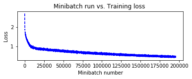
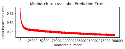
$ nvidia-smi
Sun Oct 29 19:43:46 2017
+-----------------------------------------------------------------------------+
| NVIDIA-SMI 384.90                 Driver Version: 384.90                    |
|-------------------------------+----------------------+----------------------+
| GPU  Name        Persistence-M| Bus-Id        Disp.A | Volatile Uncorr. ECC |
| Fan  Temp  Perf  Pwr:Usage/Cap|         Memory-Usage | GPU-Util  Compute M. |
|===============================+======================+======================|
|   0  Tesla K80           Off  | 0000F196:00:00.0 Off |                    0 |
| N/A   57C    P0    56W / 149W |    313MiB / 11439MiB |      0%      Default |
+-------------------------------+----------------------+----------------------+

+-----------------------------------------------------------------------------+
| Processes:                                                       GPU Memory |
|  GPU       PID   Type   Process name                             Usage      |
|=============================================================================|
|    0     11732      C   /home/masao/anaconda3/bin/python             300MiB |
+-----------------------------------------------------------------------------+
7. What's Next ?
CNTK 2.2 Python API をマスターするためには CNTK 2.2 Tutorials が最適で、
100 番台が初級、200 番台が中級、そして 300 番台が上級と区分けされています。
200 番台については特に依存関係はないようですので、興味がある分野のチュートリアルに取り組まれるのが良いでしょう。
以上