はじめに

TensorFlow2 + Keras を利用した画像分類（Google Colaboratory 環境）についての勉強メモ（第6弾）です。題材は、ド定番である手書き数字画像（MNIST）の分類です。

TensorFlow2 + Keras による画像分類に挑戦シリーズ

前回は、あらかじめ MNIST で用意されている手書き数字イメージを使って予測（分類）を行ないました。今回は、自分で用意した画像を使って、学習済みにモデルに分類をさせてみたいと思います。また、その際に要求されるリサイズやトリミングなどの前処理に関するPythonプログラム（Pillowライブラリを利用）なども解説していきたいと思います。

手書き数字画像の作成

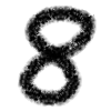
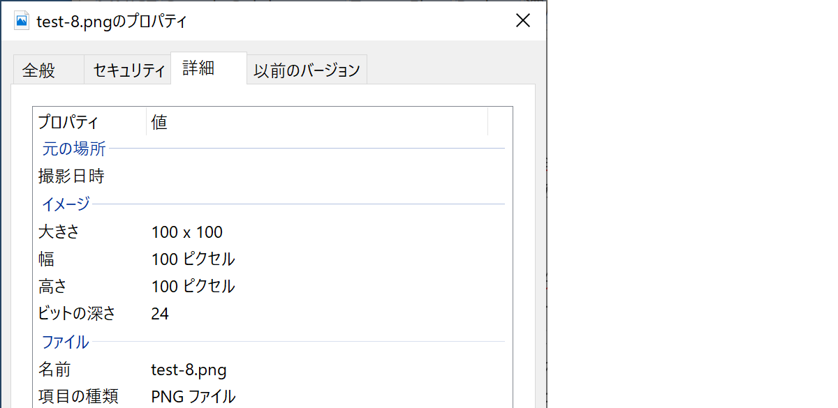
ペイントで 100 $\times$100 pixel のサイズで「8」の手書き文字を作成して、カラー（RGB）の PNGファイルとして保存しました。名前は test-8.png としました。

Google Colab. に画像ファイルをアップロード

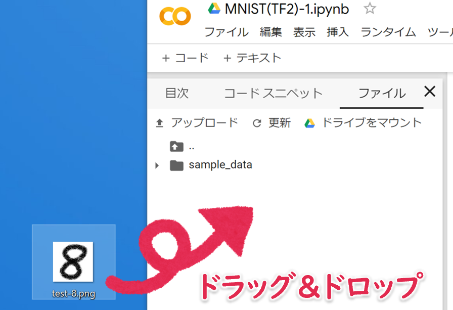
次のように、Google Colab. のサイドメニューのファイルタブをアクティブにして、デスクトップからドラッグ＆ドロップすればアップロードすることができます。アップロードしたファイルは一定時間で削除されます。

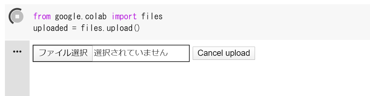
また、次のようにコードセルを書いて実行すれば、ファイル選択ダイアログを使って同様にアップロードすることができます。

アップロードされたファイル（test-8.png）の絶対パスは /content/test-8.png となります。また、カレントディレクトリは /content なので、単に test-8.png だけでもアクセスすることができます。

なお、GoogleDriveをマウントして、それを参照することもできます。詳しくは、Google Colaboratory（初利用からファイルの読込みまで）@Qiita を参照してください。

画像ファイルの読込み・内容の確認

アップロードした画像ファイルを読み込んで、内容確認のために表示します。なお、画像は Pillow（PIL Fork）を利用して扱います。わずか3行です。

import PIL.Image as Image
img = Image.open('test-8.png')
display(img)

学習済みモデルに入力可能な形式に変換

学習済みモデルに入力するためには、次の前処理が必要になります。

グレースケール画像にする。
28 $\times$28 pixel にリサイズする。
numpy.ndarray 型の2次元配列にする。
白が「0.0」、黒が「1.0」になるようにする。

次のようなコードで上記の前処理ができます。注意すべき点は、通常の256段階グレースケール画像は、白が「255」、黒が「0」なので、それを反転させる必要があるということです。

import numpy as np
import PIL.Image as Image
import matplotlib.pyplot as plt

img = Image.open('test-8.png')

img = img.convert('L')             # 1. グレースケールに変換
img = img.resize((28,28))          # 2. 28x28にリサイズ
x_sample = np.array(img)           # 3. numpy.ndarray型に変換
x_sample = 1.0 - x_sample / 255.0  # 4. 反転・正規化
y_sample = 8  # 正解データ

# 確認出力
print(f'x_sample.type = {type(x_sample)}')
print(f'x_sample.shape = {x_sample.shape}')
plt.figure()
plt.imshow(x_sample,vmin=0.,vmax=1.,cmap='Greys')
plt.show()

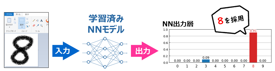
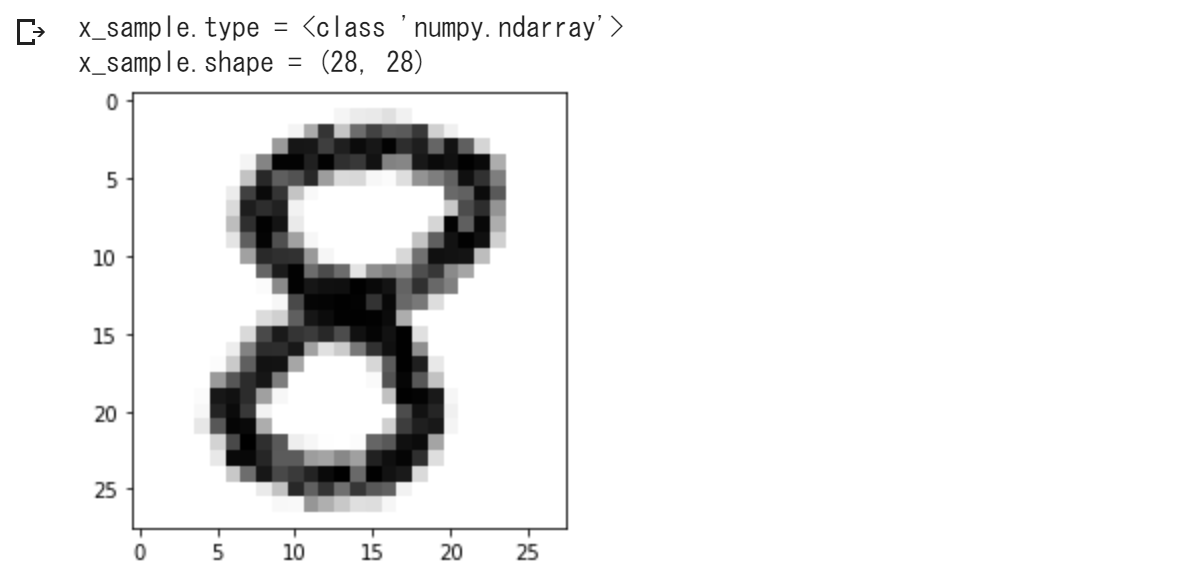
実行結果は、次のようになります。

この x_sample について、学習済みモデルで予測を行なって、第4回で示したプログラムで予測結果レポートを作成してあげると、次のようになります。

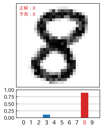
いい感じに予測（分類）を行なうことができました。

再掲：予測結果レポート作成のプログラム

基本的には、第4回で示したプログラムと同じですが、x_sampleに単体の入力データ、y_sampleに正解データ、model に学習済みモデルが格納されている前提に書き換えています。

matplotlib_日本語出力準備処理

!pip install japanize-matplotlib
import japanize_matplotlib

import numpy as np
import matplotlib.pyplot as plt
import matplotlib.patheffects as pe 
import matplotlib.transforms as ts 

s_sample = model.predict(np.array([x_sample]))[0] # 予測（分類）

fig, ax = plt.subplots(nrows=2,figsize=(3,4.2), dpi=120, 
                       gridspec_kw={'height_ratios': [3, 1]})

plt.subplots_adjust(hspace=0.05)

# 上側に手書き数字のイメージを表示
ax[0].imshow(x_sample,interpolation='nearest',vmin=0.,vmax=1.,cmap='Greys')
ax[0].tick_params(axis='both', which='both', left=False, 
                  labelleft=False, bottom=False, labelbottom=False)

# 正解値と予測値を左上に表示
t = ax[0].text(0.5, 0.5, f'正解：{y_sample}',
               verticalalignment='top', fontsize=9, color='tab:red')
t.set_path_effects([pe.Stroke(linewidth=2, foreground='white'), pe.Normal()])
t = ax[0].text(0.5, 2.5, f'予測：{s_sample.argmax()}', 
               verticalalignment='top', fontsize=9, color='tab:red')
t.set_path_effects([pe.Stroke(linewidth=2, foreground='white'), pe.Normal()])

# 下側にNN予測出力を表示
b = ax[1].bar(np.arange(0,10),s_sample,width=0.95)
b[s_sample.argmax()].set_facecolor('tab:red') # 最大項目を赤色に

# X軸設定
ax[1].tick_params(axis='x',bottom=False)
ax[1].set_xticks(np.arange(0,10))
t = ax[1].set_xticklabels(np.arange(0,10),fontsize=11)
t[s_sample.argmax()].set_color('tab:red') # 最大項目を赤色に

offset = ts.ScaledTranslation(0, 0.03, plt.gcf().dpi_scale_trans)
for label in ax[1].xaxis.get_majorticklabels() :
    label.set_transform(label.get_transform() + offset)

# Y軸設定
ax[1].tick_params(axis='y',direction='in')
ax[1].set_ylim(0,1)
ax[1].set_yticks(np.linspace(0,1,5))
ax[1].set_axisbelow(True)
ax[1].grid(axis='y')

前処理：画像中央に数字がない場合、汚れがある場合に対応

自分で手書き数字の画像を用意すると、次のように数字が画像の中央に位置していない場合があります。

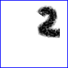
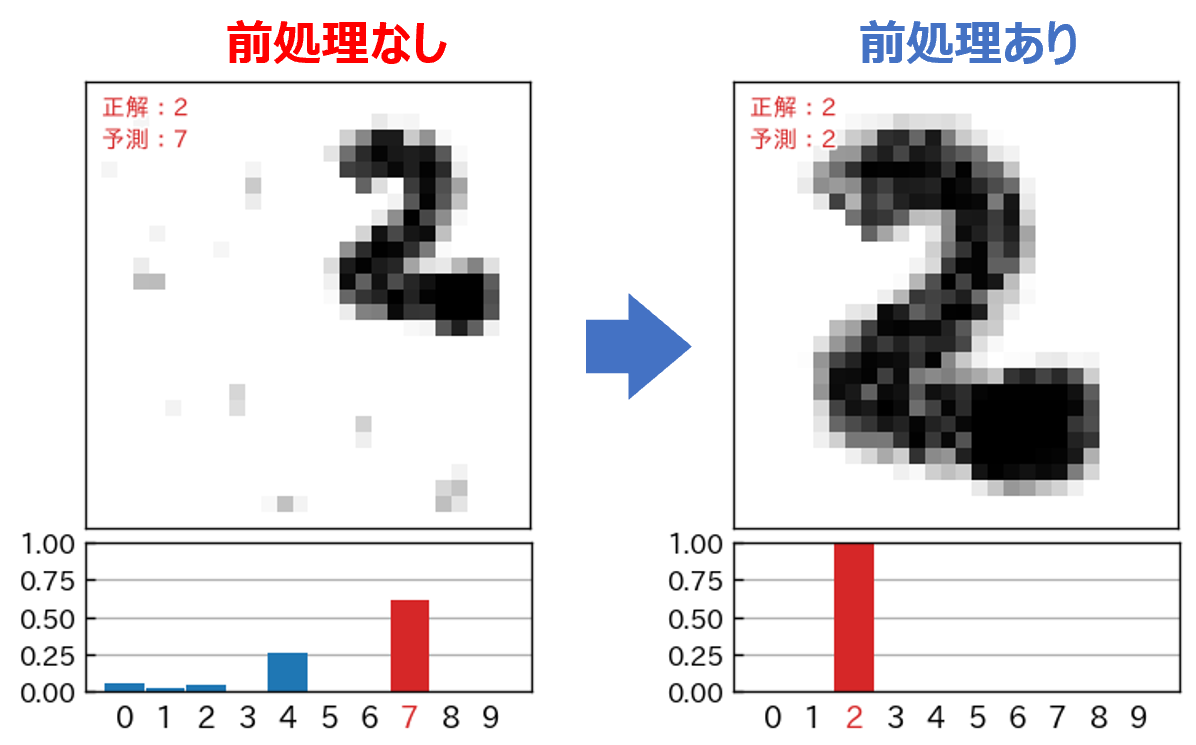
このような画像に対して、そのまま予測（分類）をかけると、次のように酷い結果となってしまいます。

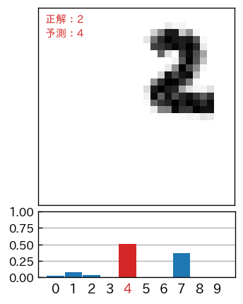
このようなことから、予測を行なう前に、文字部分を中央に移動して、さらに図の大きさに対して、正味の文字部が 90% ぐらいの大きさになるような前処理をする必要があります。また、文字以外の汚れやゴミなどを取り除く処理が必要になります。

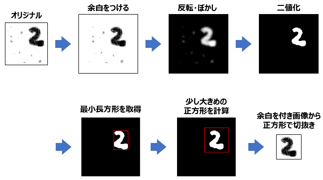
ここでは、次のような（自動化された）前処理をしたいと思います。

前処理

import numpy as np
from PIL import Image, ImageChops,ImageFilter, ImageOps, ImageDraw
import matplotlib.pyplot as plt

# 図の上下左右に指定幅の余白（白色）を付加
def add_margin(img, margin):
    w, h = img.size
    w2 = w + 2 * margin
    h2 = h + 2 * margin
    result = Image.new('L', (w2, h2), 255)
    result.paste(img, (margin, margin))
    return result

# 引数で与えられた長方形の長辺にあわせたサイズの
# 正方形（ただし、ちょっと大きくした）の正方形を計算
def to_square( rect ):
  x1, y1, x2, y2 = rect   # (x1,y1)は左上、（x2,y2)は右下の座標
  s = max( x2-x1, y2-y1 ) # 長辺の長さを取得
  s = int(s*1.3)          # 少しだけ大きく 
  nx1 = (x1+x2)/2 - s/2
  nx2 = (x1+x2)/2 + s/2
  ny1 = (y1+y2)/2 - s/2
  ny2 = (y1+y2)/2 + s/2
  return (nx1,ny1,nx2,ny2)

img = Image.open('test-2x.png')

img  = img.convert('L')
#display(img)

# 画像の上下左右に白色の余白を付ける
img  = add_margin(img,int(max(img.size)*0.2))
#display(img)

# 反転画像を作成
img2 = ImageOps.invert(img)

# ぼかしをかける
img2 = img2.filter(ImageFilter.GaussianBlur(1.5))
#display(img2)

# 二値化
img2 = img2.point(lambda p: p > 150 and 255)  
#display(img2)

# 黒色以外の最小領域（長方形）を取得
rect = img2.getbbox() 
# tmp = img2.convert('RGB')
# ImageDraw.Draw(tmp).rectangle(rect, fill=None, outline='red')
# display(tmp)

# 長方形を長辺にあわせた正方形に変換
sqr = to_square(rect)
# tmp = img2.convert('RGB')
# ImageDraw.Draw(tmp).rectangle(sqr, fill=None, outline='red')
# display(tmp)

# 正方形でトリミング
img = img.crop(sqr)
#display(img)

# 以降は前と同じ
img = img.convert('L')             # 1. グレースケールに変換
img = img.resize((28,28))          # 2. 28x28にリサイズ
x_sample = np.array(img)           # 3. numpy.ndarray型に変換
x_sample = 1.0 - x_sample / 255.0  # 4. 反転・正規化
y_sample = 2  # 正解データ

# 確認出力
print(f'x_sample.type = {type(x_sample)}')
print(f'x_sample.shape = {x_sample.shape}')
plt.figure()
plt.imshow(x_sample,vmin=0.,vmax=1.,cmap='Greys')
plt.show()

前処理せずに予測分類した場合と、前処理してから予測分類した場合についての結果の比較です。予測モデルについてあれこれ試行錯誤する以前に前処理が重要であることを改めて実感します。

次回

だいぶ外堀は埋めたので、いよいよニューラルネットワークのモデル構築について勉強していきたいと思います。

TensorFlow2 + Keras による画像分類に挑戦6 ～自分で用意した画像の前処理・分類をしてみる～