Other References
-
Environmental Setting
https://qiita.com/tanakataiki/items/40f54b3851c2ed3e09ec -
Unity&C Sharp
https://qiita.com/tanakataiki/items/fbb3a4782add01d73428 -
Performance
https://qiita.com/tanakataiki/items/94c7778341a40438cc99
学習率減衰
tf.train.polynomial_decay
decayed_learning_rate = (learning_rate - end_learning_rate) *(1 - global_step / decay_steps) ^ (power) + end_learning_rateで定義されているので,Polinomial decay chartを作ってみた.
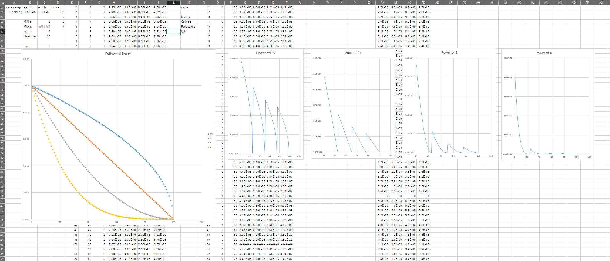
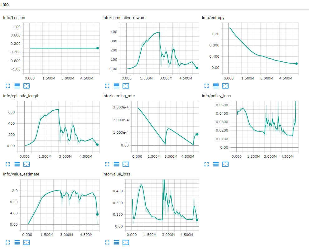
学習率が低すぎるとLocalMinimumに陥りやすいみたいです.
DecayのCycleをTrueにしたとき,3MあたりでRewardが0に近い値になってますね.
Deepmimic Hyperパラメータ
ここからが実装編
学習率設定,Epsilon設定,エントロピーの制御係数betaはCreate PPO Optimizer内で定義している.
以下は学習率は初期値1e-4,終値1e-8でTrainPolinomialDecayにて定義している時の例.
ML Agentの初期最適化関数はAdamだが,DeepmimicではMomentum OptimizerのMomentum=0.9 を使用しています.
    self.returns_holder = tf.placeholder(shape=[None], dtype=tf.float32, name='discounted_rewards')
    self.advantage = tf.placeholder(shape=[None, 1], dtype=tf.float32, name='advantages')
    self.learning_rate = tf.train.polynomial_decay(lr, self.global_step, max_step, 1e-8, power=1.0,cycle=False)
    self.old_value = tf.placeholder(shape=[None], dtype=tf.float32, name='old_value_estimates')
    decay_epsilon = tf.train.polynomial_decay(epsilon, self.global_step, max_step, 0.1, power=1.0)
    decay_beta = tf.train.polynomial_decay(beta, self.global_step, max_step, 1e-5, power=1.0)
    optimizer = tf.train.AdamOptimizer(learning_rate=self.learning_rate)
    #optimizer = tf.train.MomentumOptimizer(learning_rate=self.learning_rate,momentum=0.9)
tf.train.polinomial_decayの設定は,(初期値,現在のステップ,ステップ数,終値,乗数)となっています.
また,今はまだ実装できていないのですが,VisualObservationを入れた時,ネットワーク構造が変わることに注意.
ML-agentsのDefaultネットワーク構造はVisualObservationの値を畳み込み.VectorObservationの値をFullyConnectedしてからConcatしているが,DeepmimicはVisualObservationを含めてFullyConnectedしています.
About Code
Optimizer
optimizerについてです.
def create_ppo_optimizer(self, probs, old_probs, value, entropy, beta, epsilon, lr, max_step):
    """
    :probs: 現在の方策確率
    :param old_probs: 過去の方策確率
    :value: Valueの予測
    :beta: Entropy の規制強さ
    :entropy: 現在の方策のエントロピー
    :epsilon: ランダムな方策をとる閾値
    :lr: 学習率
    :max_step: 学習ステップの最大値.
    """

    self.returns_holder = tf.placeholder(shape=[None], dtype=tf.float32, name='discounted_rewards')
    self.advantage = tf.placeholder(shape=[None, 1], dtype=tf.float32, name='advantages')
    self.learning_rate = tf.train.polynomial_decay(lr, self.global_step, max_step, end_lr, power=1.0)
    self.old_value = tf.placeholder(shape=[None], dtype=tf.float32, name='old_value_estimates')

    decay_epsilon = tf.train.polynomial_decay(epsilon, self.global_step, max_step, 0.1, power=1.0)
    decay_beta = tf.train.polynomial_decay(beta, self.global_step, max_step, end_beta, power=1.0)


    optimizer = tf.train.MomentumOptimizer(learning_rate=self.learning_rate,momentum=0.9)
    clipped_value_estimate = self.old_value + tf.clip_by_value(tf.reduce_sum(value, axis=1) - self.old_value,
                                                               - decay_epsilon, decay_epsilon)

    v_opt_a = tf.squared_difference(self.returns_holder, tf.reduce_sum(value, axis=1))
    v_opt_b = tf.squared_difference(self.returns_holder, clipped_value_estimate)
    self.value_loss = tf.reduce_mean(tf.dynamic_partition(tf.maximum(v_opt_a, v_opt_b), self.mask, 2)[1])

    # Here we calculate PPO policy loss. In continuous control this is done independently for each action gaussian
    # and then averaged together. This provides significantly better performance than treating the probability
    # as an average of probabilities, or as a joint probability.
    r_theta = tf.exp(probs - old_probs)
    p_opt_a = r_theta * self.advantage
    p_opt_b = tf.clip_by_value(r_theta, 1.0 - decay_epsilon, 1.0 + decay_epsilon) * self.advantage
    self.policy_loss = -tf.reduce_mean(tf.dynamic_partition(tf.minimum(p_opt_a, p_opt_b), self.mask, 2)[1])
    self.loss = alpha_pi*self.policy_loss + alpha_v * self.value_loss - decay_beta * tf.reduce_mean(tf.dynamic_partition(entropy, self.mask, 2)[1])
    self.update_batch = optimizer.minimize(self.loss)
actorとcriticを共有して-lossの最小化を行う.
実際の
ActorはpolicyのLossとEntrophy
CriticはvalueのLoss
    self.actor_loss =  (self.policy_loss- decay_beta * tf.reduce_mean(tf.dynamic_partition(entropy, self.mask, 2)[1]))
    self.critic_loss = 20 * 0.5 * self.value_loss
    self.loss=self.actor_loss+self.critic_loss
A3C,PPOあたりからActorとCriticのネットワークを共有しているはずなのに,
DeepmimicではActorとCriticのネットワークを個別に作成している.
build net actor とbuild net_criticの二つのネットワークを作成している.
また,Optimizer,loss,updateなども個別に行われている.
https://github.com/xbpeng/DeepMimic/blob/8d2a2e4e0a50d15dfee5606e7fda6c6b3bbed518/learning/pg_agent.py#L138
deepmimicのActor step sizeが1e-3,critic step sizeが1e-2なので,もともとのデフォルトの値に係数を掛けた.
Deepmimic:https://github.com/xbpeng/DeepMimic/blob/8d2a2e4e0a50d15dfee5606e7fda6c6b3bbed518/learning/ppo_agent.py#L125
AI GYM: https://github.com/openai/gym
報酬のクリッピング
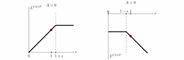
方策の勾配が以下のように極端に大きい場合以下のようにクリッピングすることによって勾配の極端な更新を防ぐことができる.
上記のtf clip by valueで報酬がクリッピングされている.
$$\frac{\pi_{\theta}(a_{t}|s_{i})}{\pi_{\theta_{old}}(a_{t}|s_{i})}>10\rightarrow \frac{\pi_{\theta}(a_{t}|s_{i})}{\pi_{\theta_{old}}(a_{t}|s_{i})}=1+\epsilon$$
p_opt_b = tf.clip_by_value(r_theta, 1.0 - decay_epsilon, 1.0 + decay_epsilon) * self.advantage
NetWork
def create_vector_observation_encoder(observation_input, h_size, activation, num_layers, scope,                                          reuse):
    """
    :reuse: 同じスコープ内でウェイトを共有するかどうか.
    :scope: Graph scope for the encoder ops.
    :observation_input: Observation.
    :h_size: 隠れ層の大きさ.
    :activation: 活性化関数.
    :num_layers: 隠れ層の数.
    :return: 隠れ層のテンソル.
    """
    with tf.variable_scope(scope):
        hidden = observation_input
        hidden = c_layers.fully_connected(hidden, h_size, activation_fn=tf.nn.relu, reuse=reuse)
        hidden = c_layers.fully_connected(hidden, int(h_size/2), activation_fn=tf.nn.relu, reuse=reuse)

        return hidden
2層目の隠れ層を半分に削減して全結合するスタイル.

Actor-Critic
Q学習やDQNなどはその先得られるであろう報酬の合計を時間割引した報酬の合計を用いて学習していた.
ValueBased・・・Value関数を用いた強化学習
Policy-Based・・・状態$s$から隠れ層を介して行動$a$を求める
Actor-CriticはValueBasedとPolicy-Basedの組み合わせによってなり立っており,
ActorはActionSpaceの出力.
Critic側はValueの出力を行う.
1ステップ先までのAdvantageを用いたCritic側の$V_{s}$は以下のようにネットワークを更新する.
$$V_{s}\rightarrow r_{t}+\gamma\cdot r_{t+1}+\gamma\cdot V_{s_{n}}$$
また,Actor側の更新はPolicyGradientにより以下の値を最大化すればよい
$$log[\pi_{\theta(a|s)}\cdot A_{t}]$$
ここで$A_{t}=R_{t}-V_{s}$であり,パラメータ更新の際は$A_{t}$は定数として扱う.
Update
割引された報酬,予測報酬,Advantage,行動確率をDictionaryにfeedしてモデルグラフを用いてUpdateを実行する場所
def update(self, mini_batch, num_sequences):
    """
    :param num_sequences: バッチ内の試行回数.
    :param mini_batch: 経験 batch.
    :return: Updateのアウトプット.
    """
    feed_dict = {self.model.batch_size: num_sequences,
                 self.model.sequence_length: self.sequence_length,
                 self.model.mask_input: mini_batch['masks'].flatten(),
                 self.model.returns_holder: mini_batch['discounted_returns'].flatten(),
                 self.model.old_value: mini_batch['value_estimates'].flatten(),
                 self.model.advantage: mini_batch['advantages'].reshape([-1, 1]),
                 self.model.all_old_log_probs: mini_batch['action_probs'].reshape(
                     [-1, sum(self.model.act_size)])}
    if self.use_continuous_act:
        feed_dict[self.model.output_pre] = mini_batch['actions_pre'].reshape(
            [-1, self.model.act_size[0]])
    else:
        feed_dict[self.model.action_holder] = mini_batch['actions'].reshape(
            [-1, len(self.model.act_size)])
        if self.use_recurrent:
            feed_dict[self.model.prev_action] = mini_batch['prev_action'].reshape(
                [-1, len(self.model.act_size)])
        feed_dict[self.model.action_masks] = mini_batch['action_mask'].reshape(
            [-1, sum(self.brain.vector_action_space_size)])
    if self.use_vec_obs:
        feed_dict[self.model.vector_in] = mini_batch['vector_obs'].reshape(
            [-1, self.vec_obs_size])
        if self.use_curiosity:
            feed_dict[self.model.next_vector_in] = mini_batch['next_vector_in'].reshape(
                [-1, self.vec_obs_size])
    if self.model.vis_obs_size > 0:
        for i, _ in enumerate(self.model.visual_in):
            _obs = mini_batch['visual_obs%d' % i]
            if self.sequence_length > 1 and self.use_recurrent:
                (_batch, _seq, _w, _h, _c) = _obs.shape
                feed_dict[self.model.visual_in[i]] = _obs.reshape([-1, _w, _h, _c])
            else:
                feed_dict[self.model.visual_in[i]] = _obs
        if self.use_curiosity:
            for i, _ in enumerate(self.model.visual_in):
                _obs = mini_batch['next_visual_obs%d' % i]
                if self.sequence_length > 1 and self.use_recurrent:
                    (_batch, _seq, _w, _h, _c) = _obs.shape
                    feed_dict[self.model.next_visual_in[i]] = _obs.reshape([-1, _w, _h, _c])
                else:
                    feed_dict[self.model.next_visual_in[i]] = _obs
    if self.use_recurrent:
        mem_in = mini_batch['memory'][:, 0, :]
        feed_dict[self.model.memory_in] = mem_in
    self.has_updated = True
    run_out = self._execute_model(feed_dict, self.update_dict)
    return run_out
TD学習(Temporal Difference Learning)
TD学習は,現在の推定値を学習中の目標値として使用することで問題を解いていく手法である。
ベルマン方程式は、状態遷移確率が未知の場合、そのまま解くことはできない.そこで,状態遷移確率は実際に観測する(サンプリングする)ことによって,確率分布を近似し,ベルマン方程式を扱う.
以下のようにValue関数の推定値を更新していく手法がTD($\lambda$)法である.
$$V_{t+1}\leftarrow (1-\alpha_{t})V_{t}(s_{t})+\alpha_{t}(r_{t+1}+\gamma V_{t}(s_{t+1})))$$
現在の値$V_{t}(s_{t})$と目標値$R_{t+1}+\gamma V_{t}(s_{t+1})$との内分によって推定値を更新していくのがこの手法であり,TD誤差として$\delta_{t}$を以下のように定義することで
TD誤差を小さくする方向に更新するアルゴリズムとして捉えることもできる.
$$\delta_{t}=(r_{t+1}+\gamma V_{t}(s_{t+1})-V_{t}(s_{t}))$$
$$V_{t+1}(s_{t})\leftarrow V_{t}(s_{t})+\alpha_{t}\delta_{t}$$
$\delta_{t}$は目標値と現在の値の差分である.
ということで以下のコードでValue関数をEstimateする.
Value Estimate
Valueの予測のための関数
def get_value_estimate(self, brain_info, idx):
    """
    :brain_info: 推定量の標本分布を予測のために使用.
    :idx: AgentのID
    :return: Valueの予測.
    """
    feed_dict = {self.model.batch_size: 1, self.model.sequence_length: 1}  # type:
    for i in range(len(brain_info.visual_observations)):
        feed_dict[self.model.visual_in[i]] = [brain_info.visual_observations[i][idx]]
    if self.use_vec_obs:
        feed_dict[self.model.vector_in] = [brain_info.vector_observations[idx]]
    if self.use_recurrent:
        if brain_info.memories.shape[1] == 0:
            brain_info.memories = self.make_empty_memory(len(brain_info.agents))
        feed_dict[self.model.memory_in] = [brain_info.memories[idx]]
    if not self.use_continuous_act and self.use_recurrent:
        feed_dict[self.model.prev_action] = brain_info.previous_vector_actions[idx].reshape(
            [-1, len(self.model.act_size)])
    value_estimate = self.sess.run(self.model.value, feed_dict)
    return value_estimate
Discount Reward
割引報酬γだけ先の報酬が割り引かれる.
def discount_rewards(r, gamma=0.99, value_next=0.0):
    """
    Computes discounted sum of future rewards for use in updating value estimate.
    :param r: List of rewards.
    :param gamma: Discount factor.
    :param value_next: T+1 value estimate for returns calculation.
    :return: discounted sum of future rewards as list.
    """
    discounted_r = np.zeros_like(r)
    running_add = value_next
    for t in reversed(range(0, r.size)):
        running_add = running_add * gamma + r[t]
        discounted_r[t] = running_add
    return discounted_r
AdvantageとGAE(Generalized Advantage Estimator)
報酬$r_{t}$,状態$s$,時間割引率$\gamma$とすると,Terminationが起こった時の状態$s$ステップ$t$では推定収益$A_{t}$は以下のようになる
$$A_{(s,a)}\rightarrow r_{t}$$
時間割引率$\gamma$はアドバンテージ関数の考慮具合を変更するための関数であり、1度実装するとパラメータ設定だけで変更できるので、generalizedと呼ばれている。
A3Cでは$\lambda=1$,PPOでは$\lambda=0.95$が使われている。
この終端からさかのぼればAdvantage関数が確からしくなっていく.
Advantageは関数の更新をNステップ先まで動かして更新しようというもの
2ステップ先までの更新は
$$A_{(s,a)}\rightarrow r_{t}+\gamma\cdot r_{t+1}+\gamma^{2}\cdot max[A_{(s_{n},a)}]$$
3ステップ先は
$$A_{(s,a)}\rightarrow r_{t}+\gamma\cdot r_{t+1}+\gamma^{2}\cdot r_{t+2}+\gamma^{3}・max[A_{(s_{n},a)}]$$
4ステップ先は
$$A_{(s,a)}\rightarrow r_{t}+\gamma\cdot r_{t+1}+\gamma^{2}\cdot r_{t+2}+\gamma^{3}\cdot r_{t+3}+\gamma^{4}・max[A_{(s_{n},a)}]$$
5ステップ先は$$...ま,いいか$$
各タイムステップ$t$での状態$s_{t}$において行動$a_{t}$を行い報酬$r_{t}$をもらい次のタイムステップ
$t+1$における状態$s_{t+1}$において行動$a_{t+1}$を行い報酬$r_{t+1}$を得る
GAE
GAEの関数Valueの予測値の誤差を最小化する関数
def get_gae(rewards, value_estimates, value_next=0.0, gamma=0.99, lambd=0.95):
    """
    Computes generalized advantage estimate for use in updating policy.
    :param rewards: list of rewards for time-steps t to T.
    :param value_next: Value estimate for time-step T+1.
    :param value_estimates: list of value estimates for time-steps t to T.
    :param gamma: Discount factor.
    :param lambd: GAE weighing factor.
    :return: list of advantage estimates for time-steps t to T.
    """
    value_estimates = np.asarray(value_estimates.tolist() + [value_next])
    delta_t = rewards + gamma * value_estimates[1:] - value_estimates[:-1]
    advantage = discount_rewards(r=delta_t, gamma=gamma * lambd)
    return advantage
Update Policy
PolicyのUpdate
trainer/policy.py
batch_size:4096
buffer_size:batch_size*50
sequence_length:16
これで
n_sequence=(batch_size/sequence_length)=minibatch_size=256
になりDeepmimicのParameterと合わせることができた.
num_epoch:32
sequenceごとにbatch sizeを分割し,
def update_policy(self):
    """
    Uses training_buffer to update the policy.
    """
    n_sequences = max(int(self.trainer_parameters['batch_size'] / self.policy.sequence_length), 1)
    value_total, policy_total, forward_total, inverse_total = [], [], [], []
    advantages = self.training_buffer.update_buffer['advantages'].get_batch()
    self.training_buffer.update_buffer['advantages'].set(
        (advantages - advantages.mean()) / (advantages.std() + 1e-10))
    num_ = self.trainer_parameters['num_epoch']
    for k in range(num_epoch):
        self.training_buffer.update_buffer.shuffle()
        buffer = self.training_buffer.update_buffer
        for l in range(len(self.training_buffer.update_buffer['actions']) // n_sequences):
            start = l * n_sequences
            end = (l + 1) * n_sequences
            run_out = self.policy.update(buffer.make_mini_batch(start, end), n_sequences)
            value_total.append(run_out['value_loss'])
            policy_total.append(np.abs(run_out['policy_loss']))
            if self.use_curiosity:
                inverse_total.append(run_out['inverse_loss'])
                forward_total.append(run_out['forward_loss'])
    self.stats['value_loss'].append(np.mean(value_total))
    self.stats['policy_loss'].append(np.mean(policy_total))
    if self.use_curiosity:
        self.stats['forward_loss'].append(np.mean(forward_total))
        self.stats['inverse_loss'].append(np.mean(inverse_total))
    self.training_buffer.reset_update_buffer()
Deepmimic
. Learning curves of the humanoid imitating individual motion clips. Performance is calculated as the mean return over 32 episodes. The returns are
normalized by the minimum and maximum possible return per episode. Due to the time needed to train each policy, performance statistics are collected only
from one run of the training process for the majority of skills. For the backflip and run policies, we collected statistics from 3 training runs using different
random seeds. Performance appears consistent across multiple runs, and we have observed similar behaviours for many of the other skills
Stacked Vector
Vector Observation*Stacked Vectorの数だけ取り込み,mean varianceを計算し,入力として入れていた.
def create_vector_input(self, name='vector_observation'):
    """
    Creates ops for vector observation input.
    :param name: Name of the placeholder op.
    :param vec_obs_size: Size of stacked vector observation.
    :return:
    """
    self.vector_in = tf.placeholder(shape=[None, self.vec_obs_size], dtype=tf.float32,
                                    name=name)
    if self.normalize:
        self.running_mean = tf.get_variable("running_mean", [self.vec_obs_size],
                                            trainable=False, dtype=tf.float32,
                                            initializer=tf.zeros_initializer())
        self.running_variance = tf.get_variable("running_variance", [self.vec_obs_size],
                                                trainable=False,
                                                dtype=tf.float32,
                                                initializer=tf.ones_initializer())
        self.update_mean, self.update_variance = self.create_normalizer_update(self.vector_in)

        self.normalized_state = tf.clip_by_value((self.vector_in - self.running_mean) / tf.sqrt(
            self.running_variance / (tf.cast(self.global_step, tf.float32) + 1)), -5, 5,
                                                 name="normalized_state")
        return self.normalized_state
    else:
        return self.vector_in
Architecture
Stacked VectorはFully connnected された後にflattenされるので,Stacked Vectorの数を増やすと,結果的にネットワークのInputが増える.
    for i in range(num_streams):
        visual_encoders = []
        hidden_state, hidden_visual = None, None
        if self.vis_obs_size > 0:
            for j in range(brain.number_visual_observations):
                encoded_visual = self.create_visual_observation_encoder(self.visual_in[j],
                                                                        h_size,
                                                                        activation_fn,
                                                                        num_layers,
                                                                        "main_graph_{}_encoder{}"
                                                                        .format(i, j), False)
                visual_encoders.append(encoded_visual)
            hidden_visual = tf.concat(visual_encoders, axis=1)
                visual_n_state_input=tf.concat([vector_observation_input,hidden_visual],axis=1)
                hidden_state = self.create_continuous_observation_encoder(visual_n_state_input,h_size, activation_fn, num_layers,"main_graph_{}".format(i), False)
            if hidden_state is not None and hidden_visual is not None:
                final_hidden = hidden_state
            final_hiddens.append(final_hidden)
        if deepMimicArchitecture==True and hidden_visual==None:
            if brain.vector_observation_space_size > 0:
                hidden_state = self.create_continuous_observation_encoder(vector_observation_input,h_size, activation_fn, num_layers,"main_graph_{}".format(i), False)
                final_hidden = hidden_state
            final_hiddens.append(final_hidden)
Leaning Algorithm
Policyのアップデートはbatch_size=4096の間隔で行われ,minibatch_size 256は勾配更新のタイミングでサンプルされる.
割引率$\gamma=0.95$は全てのモーションに対して行われており,$\lambda=0.95$はTD$(\lambda)$とGAE$(\lambda)$で使用されている.
likehood threshold clipping の閾値は$\epsilon=0.2$,Value関数のステップサイズ$a_{v}=10^{-2}$
Policyのステップサイズ$a_{\pi}=5\times10^{-5}$は人型とアトラス用,$a_{\pi}=2\times10^{-5}$はTrexとDragon用に使用されている.
確率的勾配降下法のMomentum法のdecay 0.9を用いておこなっており,それぞれのスキルは2日間の訓練を8CPUのパソコンで6000万サンプルの訓練により学習している.
batch_size:4096
minibatch_size:256
beta: 5.0e-3
buffer_size: 12288
epsilon: 0.2
gamma: 0.95
hidden_units: 1024->512
lambd: 0.95
learning_rate: 3.0e-4
max_steps: 60.0e6
normalize: true
num_layers: 2
これはtrainer_config.yamlで定義している.
WalkingBrain:
learning_rate: 3.0e-4
beta: 5.0e-3
num_epoch: 3
time_horizon: 1000
batch_size: 4096
buffer_size: 81920
gamma: 0.95
lambd: 0.95
max_steps: 5e6
num_layers: 2
hidden_units: 1024ー>512
ちなみにEpsilonはDefaultの0.2を踏襲している.
MachineSpec
CPU : Dual CPU Xenon v3 8core×2 RAM 128 GB
GPU : 1080Ti