目次
- 第1章 はじめに
- 第2章 パーセプトロン
- 第3章 ニューラルネットワーク
- 第4章 ニューラルネットワークの学習
- 第5章 誤差逆伝播法
- 第6章 学習に関するテクニック
- 第7章 畳み込みニューラルネットワーク
- 第8章 ディープラーニング
- 最後に
6.2.2 隠れ層のアクティベーション分布
本書とは少し違って、初期値の標準偏差を4通りに変えながらグラフを作成するようにしてみました。
// ch06/weight_init_activtion_histogram.pyのJava版です。
INDArray x = Nd4j.randn(new int[] {1000, 100}); // 1000個のデータ
int node_num = 100; // 各隠れ層のノード(ニューロン)の数
int hidden_layer_size = 5; // 隠れ層が5層
Map<Integer, INDArray> activations = new HashMap<>(); // ここにアクティベーションの結果を格納する
Map<String, Supplier<INDArray>> ws = new LinkedHashMap<>();
// 初期値の値をいろいろ変えて実験しよう!
ws.put("1.0", () -> Nd4j.randn(new int[] {node_num, node_num}).mul(1));
ws.put("0.01", () -> Nd4j.randn(new int[] {node_num, node_num}).mul(0.01));
ws.put("sqrt(1 div n)", () -> Nd4j.randn(new int[] {node_num, node_num}).mul(Math.sqrt(1.0 / node_num)));
ws.put("sqrt(2 div n)", () -> Nd4j.randn(new int[] {node_num, node_num}).mul(Math.sqrt(2.0 / node_num)));
for (String key : ws.keySet()) {
    for (int i = 0; i < hidden_layer_size; ++i) {
        if (i != 0)
            x = activations.get(i - 1);
        INDArray w = ws.get(key).get();
        INDArray a = x.mmul(w);
        // 活性化関数の種類も変えて実験しよう!
        INDArray z = Functions.sigmoid(a);
        // INDArray z = Functions.relu(a);
        // INDArray z = Functions.tanh(a);
        activations.put(i, z);
    }
    // ヒストグラムを描画
    for (Entry<Integer, INDArray> e : activations.entrySet()) {
        HistogramImage h = new HistogramImage(320, 240, -0.1, -1000, 1, 40000, 50, e.getValue());
        h.writeTo(new File(Constants.WeightImages, key + "-" + (e.getKey() + 1) + "-layer.png"));
    }
}
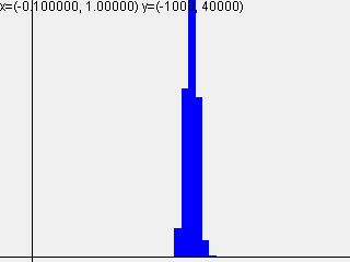
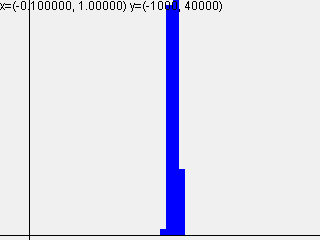
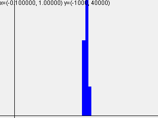
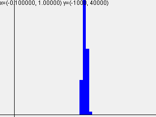
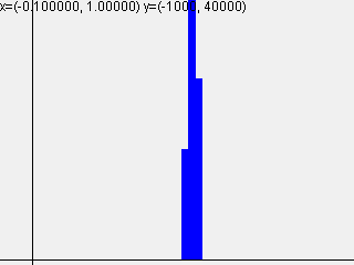
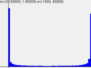
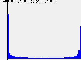
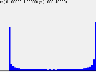
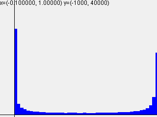
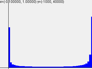
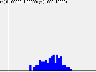
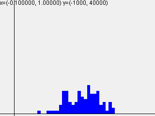
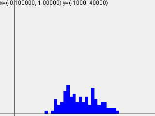
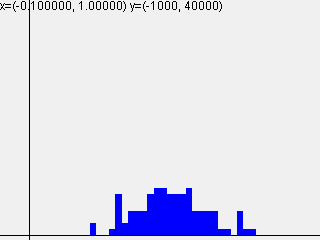
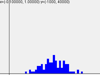
活性化関数sigmoidを使って標準偏差を変えて実行した結果は以下のようになりました。
標準偏差 = 0.01
| 1-layer | 2-layer | 3-layer | 4-layer | 5-layer |
|---|---|---|---|---|
 |
 |
 |
 |
 |
標準偏差 = 1.0
| 1-layer | 2-layer | 3-layer | 4-layer | 5-layer |
|---|---|---|---|---|
 |
 |
 |
 |
 |
標準偏差 = $\sqrt{\frac{1}{n}}$
| 1-layer | 2-layer | 3-layer | 4-layer | 5-layer |
|---|---|---|---|---|
 |
 |
 |
 |
 |
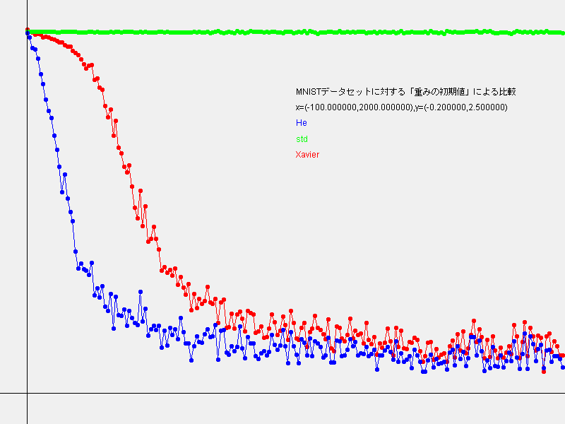
6.2.4 MNISTデータセットによる重み初期値の比較
// ch06/weight_init_compare.pyのJava版です。
MNISTImages train = new MNISTImages(Constants.TrainImages, Constants.TrainLabels);
INDArray x_train = train.normalizedImages();
INDArray t_train = train.oneHotLabels();
DataSet dataset = new DataSet(x_train, t_train);
int train_size = x_train.size(0);
int batch_size = 128;
int max_iteration = 2000;

// 1:実験の設定
Map<String, String> weight_init_types = new HashMap<>();
weight_init_types.put("std", "0.01");
weight_init_types.put("Xavier", "sigmoid");
weight_init_types.put("He", "relu");
Optimizer optimizer = new SGD(0.01);

Map<String, MultiLayerNet> networks = new HashMap<>();
Map<String, List<Double>> train_loss = new HashMap<>();
for (Entry<String, String> e : weight_init_types.entrySet()) {
    String key = e.getKey();
    String weight_init_std = e.getValue();
    networks.put(key, new MultiLayerNet(
        784, new int[] {100, 100, 100, 100}, 10, weight_init_std));
    train_loss.put(key, new ArrayList<>());
}

//2:訓練の開始
for (int i = 0; i < max_iteration; ++i) {
    DataSet sample = dataset.sample(batch_size);
    INDArray x_batch = sample.getFeatureMatrix();
    INDArray t_batch = sample.getLabels();

    for (String key : weight_init_types.keySet()) {
        MultiLayerNet network = networks.get(key);
        Params grads = network.gradicent(x_batch, t_batch);
        optimizer.update(network.params, grads);

        double loss = network.loss(x_batch, t_batch);
        train_loss.get(key).add(loss);
    }

    if (i % 100 == 0) {
        System.out.println("===========" + "iteration:" + i + "===========");
        for (String key : weight_init_types.keySet()) {
            double loss = networks.get(key).loss(x_batch, t_batch);
            System.out.println(key + ":" + loss);
        }
    }
}

// 3:グラフの描画
GraphImage graph = new GraphImage(800, 600, -100, -0.2, max_iteration, 2.5);
Map<String, Color> colors = new HashMap<>();
colors.put("std", Color.GREEN);
colors.put("Xavier", Color.RED);
colors.put("He", Color.BLUE);
double h = 1.5;
for (String key : weight_init_types.keySet()) {
    List<Double> losses = train_loss.get(key);
    graph.color(colors.get(key));
    graph.text(key, 1000, h);
    h += 0.1;
    int step = 10;
    graph.plot(0, losses.get(0));
    for (int i = step; i < max_iteration; i += step) {
        graph.line(i - step, losses.get(i - step), i, losses.get(i));
        graph.plot(i, losses.get(i));
    }
}
graph.color(Color.BLACK);
graph.text(String.format("x=(%f,%f),y=(%f,%f)",
    graph.minX, graph.maxX, graph.minY, graph.maxY), 1000, h);
h += 0.1;
graph.text("MNISTデータセットに対する「重みの初期値」による比較", 1000, h);
graph.writeTo(Constants.file(Constants.WeightImages, "weight_init_compare.png"));
}
結果のグラフは以下のようになりました。