This article is written in English. Japanese Version is here.
Introduction
Welcome to the second instalment of our structural analysis tutorial series in the age of AlphaFold2 (click here for the first instalment). This time, we will calculate the structure factor F(hkl) from a diffraction image dataset.
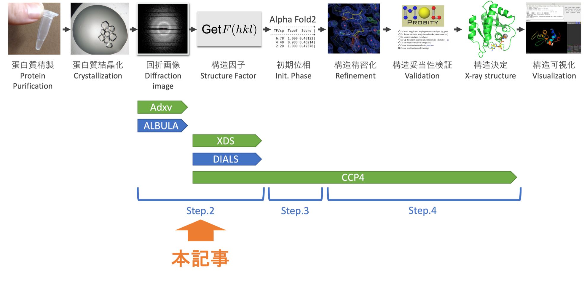
Table of Contents
- Step.0 The flow of structure determination
- Step.1 Installing analytical software
- Step.2 Checking diffraction images and calculating structure factors (this article)
- Step.3 Finding initial phases
- Step.4 Structure refinement and validation
Target Audience and Objective of this Article
This article is aimed at researchers, graduate students, and undergraduate students who are not specialists in protein X-ray crystallography. The goal is to enable you to go from diffraction images to structure determination in protein X-ray crystallography. It is assumed that you have some experience with the Bash command in a Linux environment.
We will deliver this tutorial on protein structure analysis in four instalments. This is the second instalment.
Furthermore, this article is entirely open. Whether in schools, research institutions, or companies, we hope you will spread this article and use it for educational purposes. However, copyright is not relinquished.
Computing Environment Needed for Protein X-ray Crystallographic Analysis
From my experience, the following computing environment is suitable for protein X-ray crystallographic analysis. It requires computer power, so it's important not to attempt it on a Raspberry Pi or similar device.
- OS
- Linux, such as Ubuntu, CentOS (strongly recommended)
- MacOSX
- Windows 10/11 (use either the native environment or a Linux environment on WSL2)
- CPU: > 4 cores (recommended: > 16 cores)
- Main Memory: > 16 GB (recommended: > 32 GB)
- Storage: > 50 GB (about 12 GB for software installation, data sets 20 - 30 GB/crystal)
- GPU: Not essential (recommended: equipped with a GPU)
Github Repository
We have uploaded representative files related to this tutorial to Github. We hope it will serve as a useful reference.
Step.2 Diffraction Image Verification and Structure Factor Calculation
Step.2-1 Data Preparation
In this tutorial, we will elucidate the model structure of Lysozyme, a saccharide hydrolase derived from chicken egg white, which could be considered the "Hello World" structure of protein X-ray crystallography. Obtain the diffraction image and amino acid sequence from the links below.
| Data | Download URL | Remarks |
|---|---|---|
| Diffraction Image | Integrated Resource for Reproducibility in Macromolecular Crystallography, NIH, nsls2_fmx_20161122_lys_266 | Data obtained for beamline adjustment at Beamline 17-ID-2 of the National Synchrotron Light Source in the United States. Approximately 13GB. |
| Amino Acid Sequence | UniProt, P00698 LYSC_CHICK | Click the "Download" button in the "Sequence" section and save the sequence from the 19th residue to the end in a suitable text file (for example: lysozyme.fasta). The sequence displayed in Uniprot is indeed the full length of the protein, but since the product is often sold with the 1~18 residues removed and it is crystallized in that state, we already remove it. Here is the sequence of Lysozyme from the 19th residue to the end, which you are welcome to use. |
KVFGRCELAAAMKRHGLDNYRGYSLGNWVCAAKFESNFNTQATNRNTDGSTDYGILQINSRWWCNDGRTPGSRNLCNIPCSALLSSDITASVNCAKKIVSDGNGMNAWVAWRNRCKGTDVQAWIRGCRL
Step 2-2: Reviewing the Diffraction Image
Obtaining a reliable protein structure necessitates a high-quality electron density map, $\rho (xyz)$1. A quality electron density map $\rho (xyz)$ requires a high-quality structure factor, $F(hkl)$, and the linchpin for this is the quality of the diffraction image. Therefore, verifying the quality of the diffraction image is an extremely crucial step to obtaining a quality protein structure.
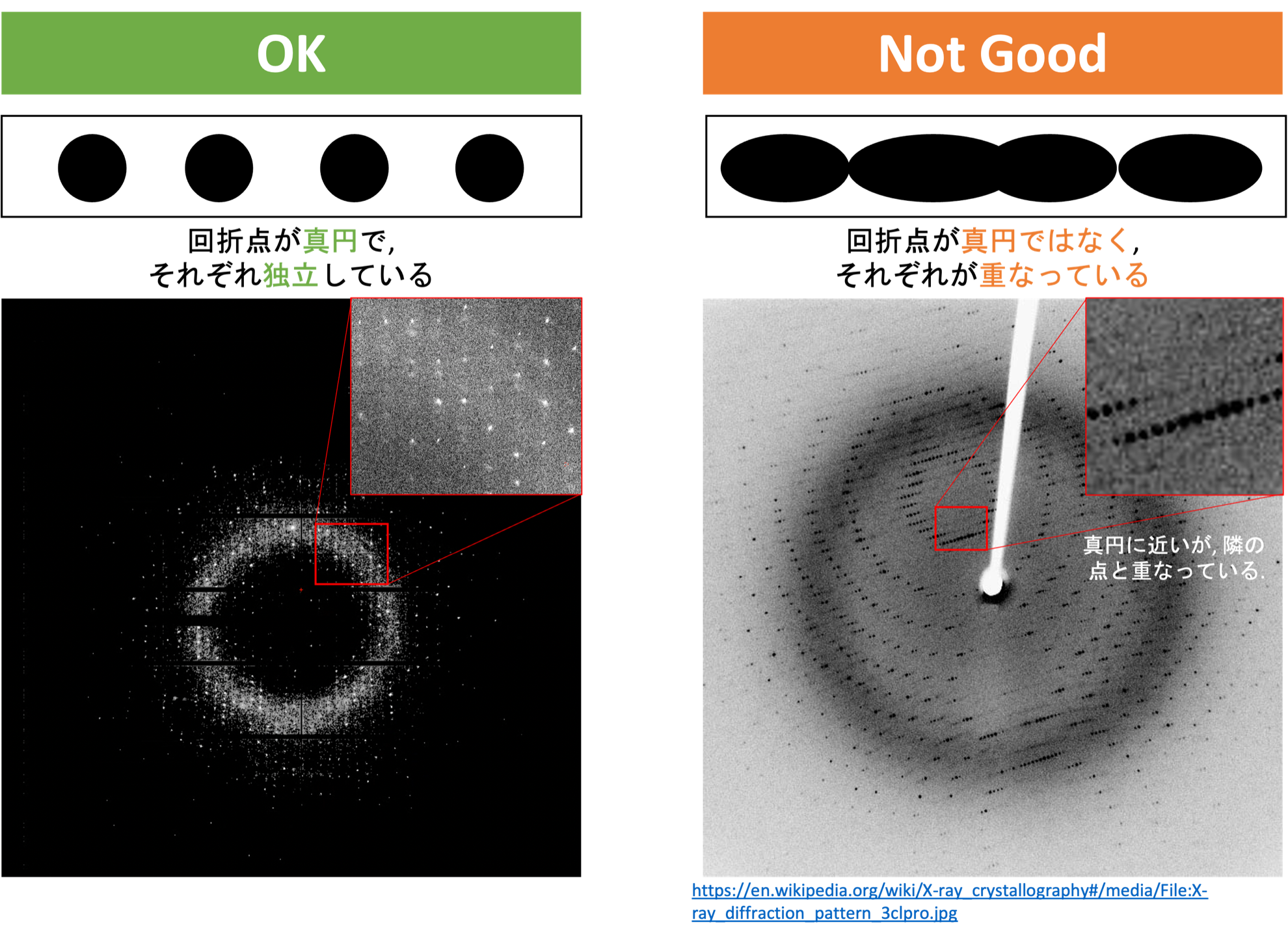
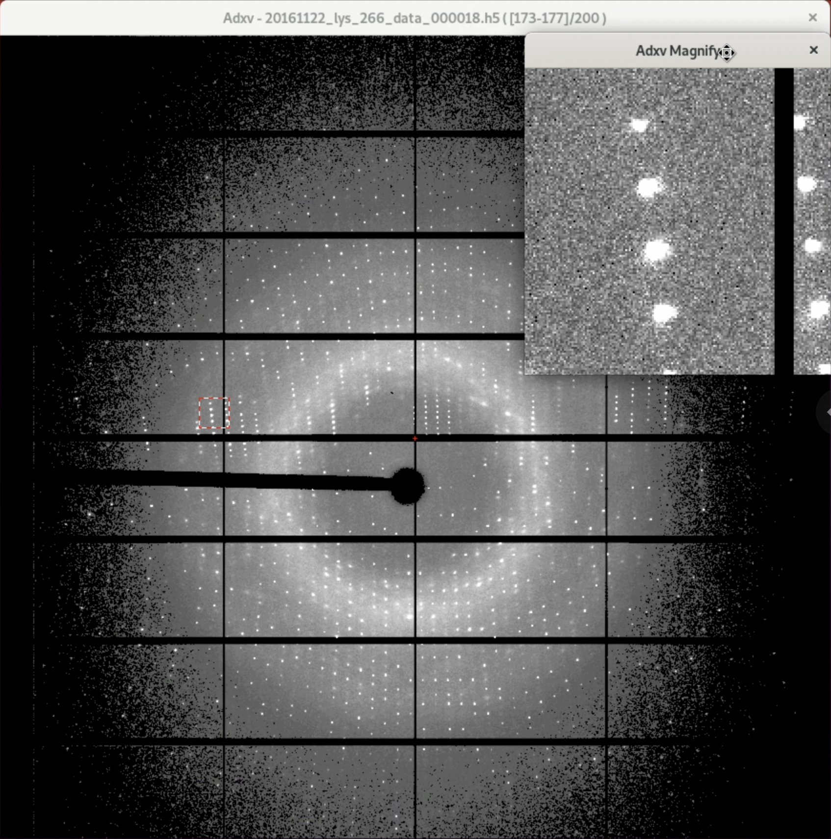
So, what exactly constitutes a good diffraction image? It is an image where the diffraction spots are nearly circular, and the spots do not overlap with each other. This is primarily what is checked in the verification of the diffraction image. An actual image is shown below.
Though we are digressing, one might ask what a diffraction image is. Not limited to protein crystals, when X-rays are irradiated on a crystal, specific diffraction phenomena occur due to the arrangement of molecules in the crystal. These phenomena are visualized on a two-dimensional detector. This is what is referred to as a diffraction image. Moreover, the experiment to obtain a diffraction image is called a "diffraction experiment." The diffraction experiment is explained in an easy-to-understand manner in this Wikipedia article and is worth referencing.
Although regularly arranged diffraction spots can be observed in a diffraction image as shown in the figure above, the positions of these diffraction spots depend on the following parameters:
- The size of the crystal's unit cell (Defined by - the lengths of the three sides $a,b,c$ and the angles $\alpha, \beta, \gamma$, these determine the Bravais lattice to which the crystal belongs)
- The wavelength of the X-rays (nm)
- The orientation of the crystal
- The distance between the crystal and the detector
- The size of the detector
To calculate the structure factor $F(hkl)$, all the above parameters need to be determined. This is mostly done automatically by software (XDS in this tutorial) in the next step, a process known as Indexing. Once all parameters are determined, it becomes clear which Miller index $hkl$ each measured diffraction spot corresponds to. The intensity of each diffraction spot is calculated by the software in a form corresponding to the Miller index $hkl$, a process known as Integration. By statistically combining these, the structure factor $F(hkl)$ is derived, a process known as Scaling. The importance of the diffraction spots being nearly circular and not overlapping is to accurately estimate the position and intensity of the diffraction spots.
Furthermore, to finally determine the model structure of the protein, it is essential to identify the space group of the crystal. While this is somewhat identified in Scaling through the extinction rule, it cannot be definitively determined without trying to solve the initial phase/protein model structure.
Step 2-3: Diffraction Image Format
Before taking a closer look at the diffraction image, let's briefly discuss the image format output from the two-dimensional detector.
With the advancement of technology, two-dimensional detectors have evolved from film --> CCD --> CMOS --> hybrid pixel, greatly improving the detection S/N ratio, resolution, and imaging speed. Since around 2014, detectors from Swiss DECTRIS have become the industry standard.
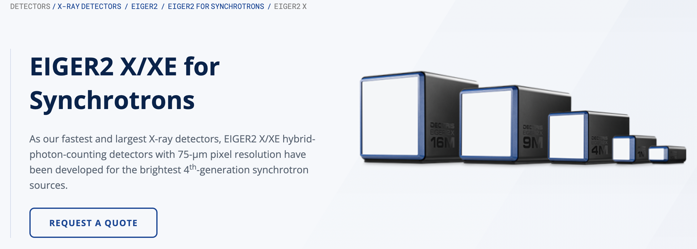
(The current flagship model, EIGER2 series made by DECTRIS. Source: https://www.dectris.com/detectors/x-ray-detectors/eiger2/eiger2-for-synchrotrons/eiger2-x/)
The diffraction image format varies depending on the two-dimensional detector. Diffraction experiments are often conducted at the dedicated beamlines of synchrotron facilities. Various types of two-dimensional detectors have been used so far. Detectors using CCD technology, which was mainstream until around 2013, took about 20-30 minutes to obtain up to 360 diffraction images per data set. The diffraction images from this era were independent image files with extensions such as "img" or "osc". However, as of 2023, the main detectors use hybrid pixel technology. These can capture up to about 3,600 diffraction images required for one data set in just 1-2 minutes. Due to this explosive increase in the number of images taken per unit of time (and the reduction in X-ray irradiation time due to the improved S/N ratio), researchers can measure many crystals in a limited beam time.
On the other hand, the output of a large number of diffraction images in a short period posed challenges in data handling2. Thus, in recent years, diffraction images are often stored in the HDF5 format, a hierarchical file container that can also be used as training data for deep learning. The diffraction images used in this tutorial are also stored in HDF5 format, integrating 200 images into a single HDF5 file.
On one hand, the rapid output of a large number of diffraction images poses data handling challenges2. Therefore, in recent years, diffraction images are often stored in HDF5 format, a hierarchical file container that can be used for deep learning training data. The diffraction images used in this tutorial are also stored in HDF5 format, consolidating 200 images into a single HDF5 file.
Step 2-4: Display and Verification of Diffraction Images
The first step is to check the diffraction images, which will initiate the protein X-ray crystal structure analysis.
- Start adxv by typing
adxvin the terminal.
$ adxv
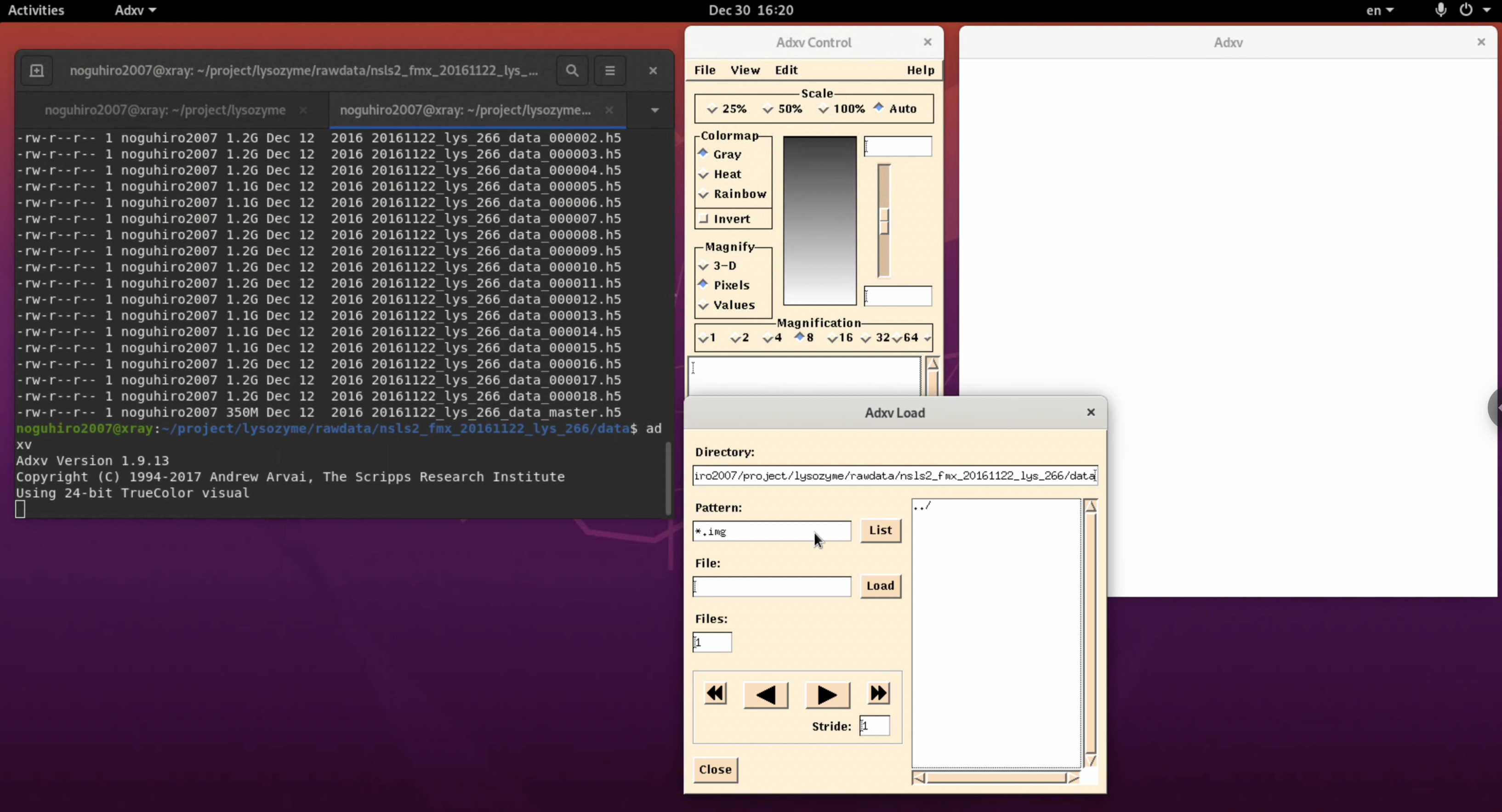
2. In the "Adxv Load" window, specify the folder containing the diffraction image files in the Directory field, change the Pattern from " *.img " to " * ", and click List.
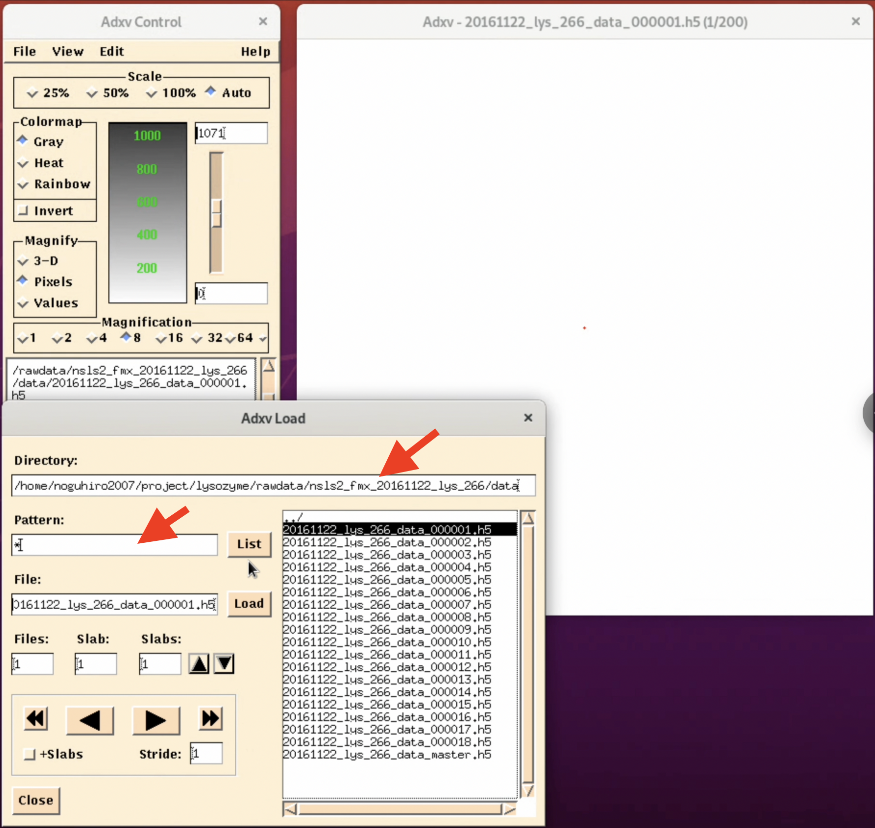
3. A file list will be displayed on the right side of the "Adxv Load" window. Here, select the image file you want to check and click Load.
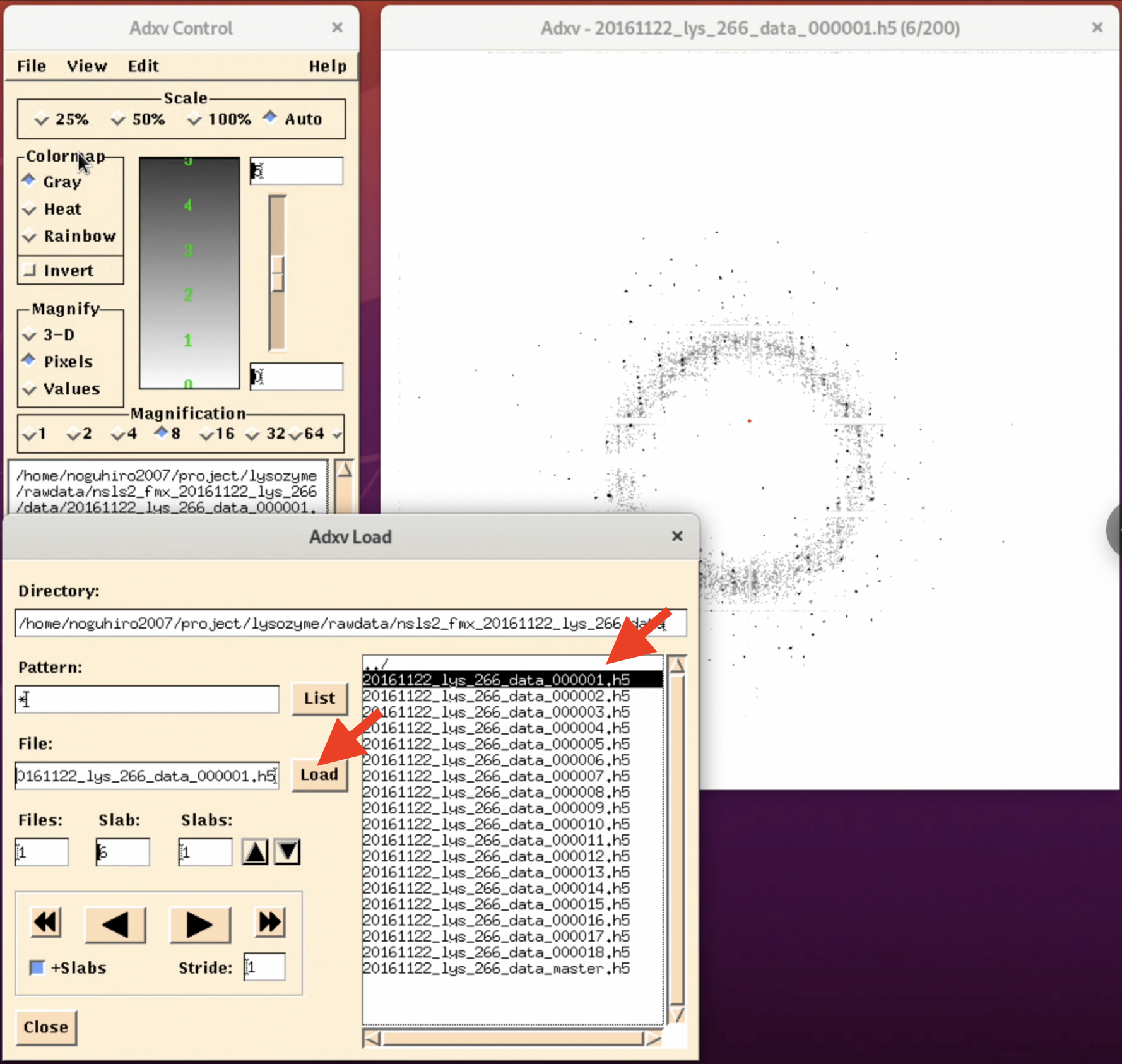
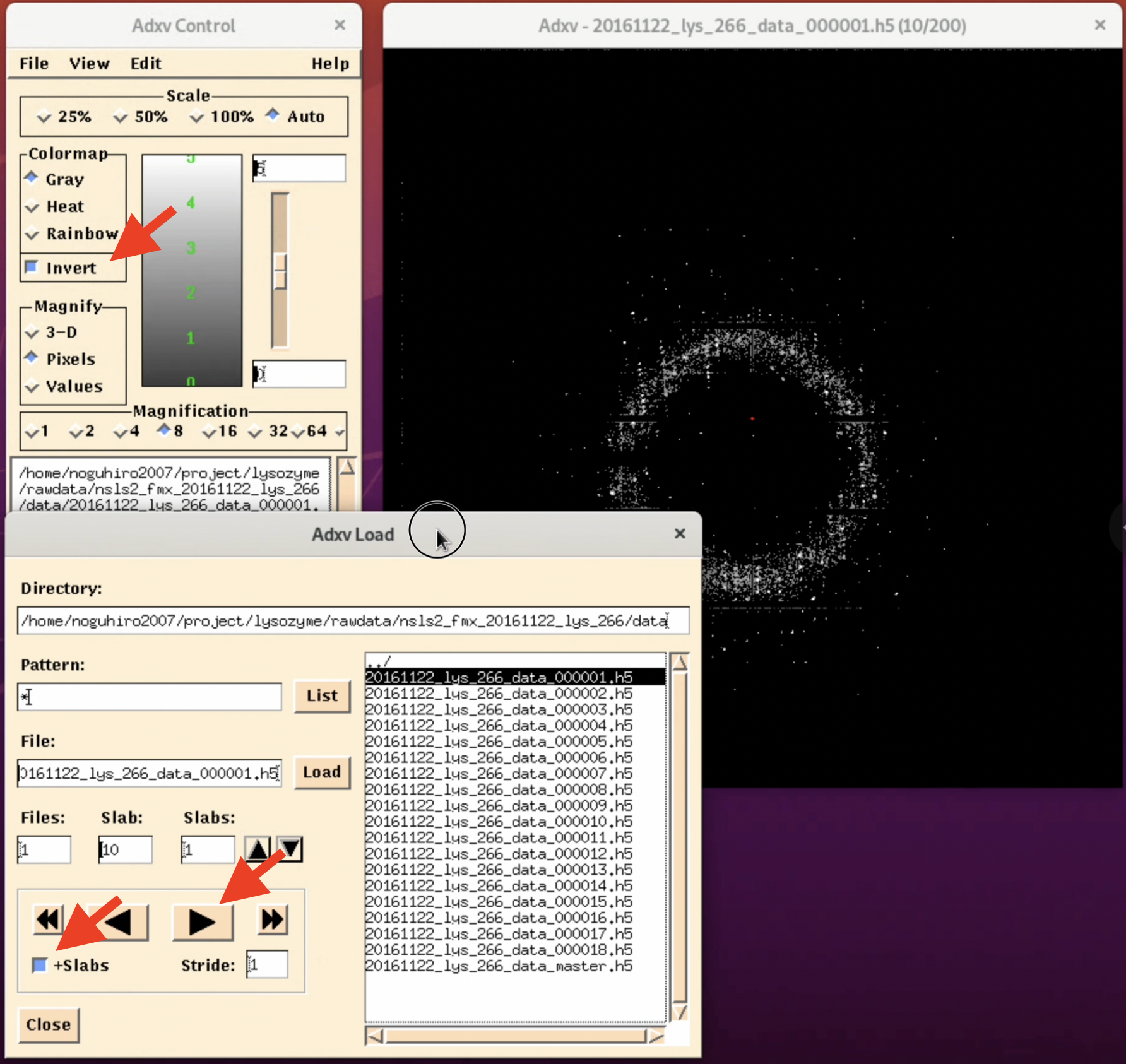
4. Adjust for better visibility. By selecting the invert button in the "Adxv Control" window, the image will be inverted, making it easier to find the outer diffraction spots (this can vary depending on the person). Also, by pressing the arrow button in the "Adxv Load" window, you can display the image of the next file. At this time, clicking "+Slabs" will allow you to see the diffraction images inside the h5 file.
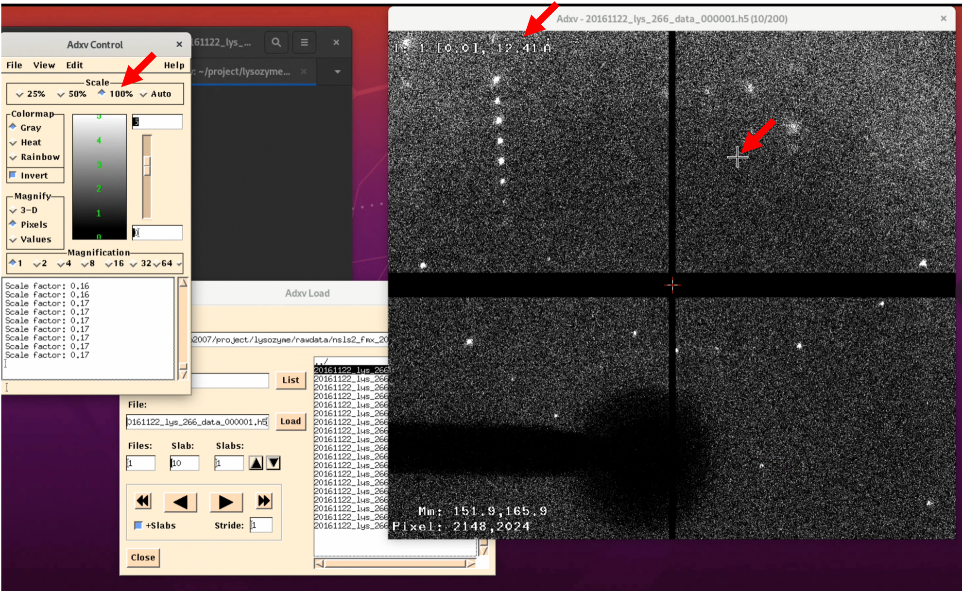
Additionally, the Scale in the "Adxv Control" is the magnification of the diffraction image, and at actual size, it will look like the image below (the actual magnification depends on the resolution of the display). Also, the "12.41 Å" in the upper left corner of the diffraction image indicates the resolution at the current location of the mouse pointer "+". The further out you go, the higher the resolution, and if there are diffraction spots there, you can obtain a more reliable structure3. There are other settings, so we recommend exploring a bit.
5. Diffraction Image Check 1: Go through all the images
Roughly check all images to ensure that diffraction spots are not missing halfway, and no diffraction spots with different patterns appear. As shown in the video below, clicking the "double-play button" will automatically play the diffraction images.
6. Diffraction Image Check 2: Check the quality of the diffraction spots
For diffraction images at 0°, +45°, +90°, +135°...and every 45°, check the quality of the diffraction spots. If the diffraction spots are round and not overlapping with each other, as shown in the figure below, there should be no problem.
Please note that the dataset used in this tutorial contains very high-quality diffraction images. We hope this will serve as a positive control when checking other diffraction images.
Step 2-5: Calculation of Structure Factors
Step 2-5-1: Processing Diffraction Images with XDS
Once the quality check of the diffraction images is completed and a general understanding of the dataset is established, we can proceed to the calculation of the structure factors $F(hkl)$.
- Type
xdsguiin the terminal to start xdsgui.
$ xdsgui
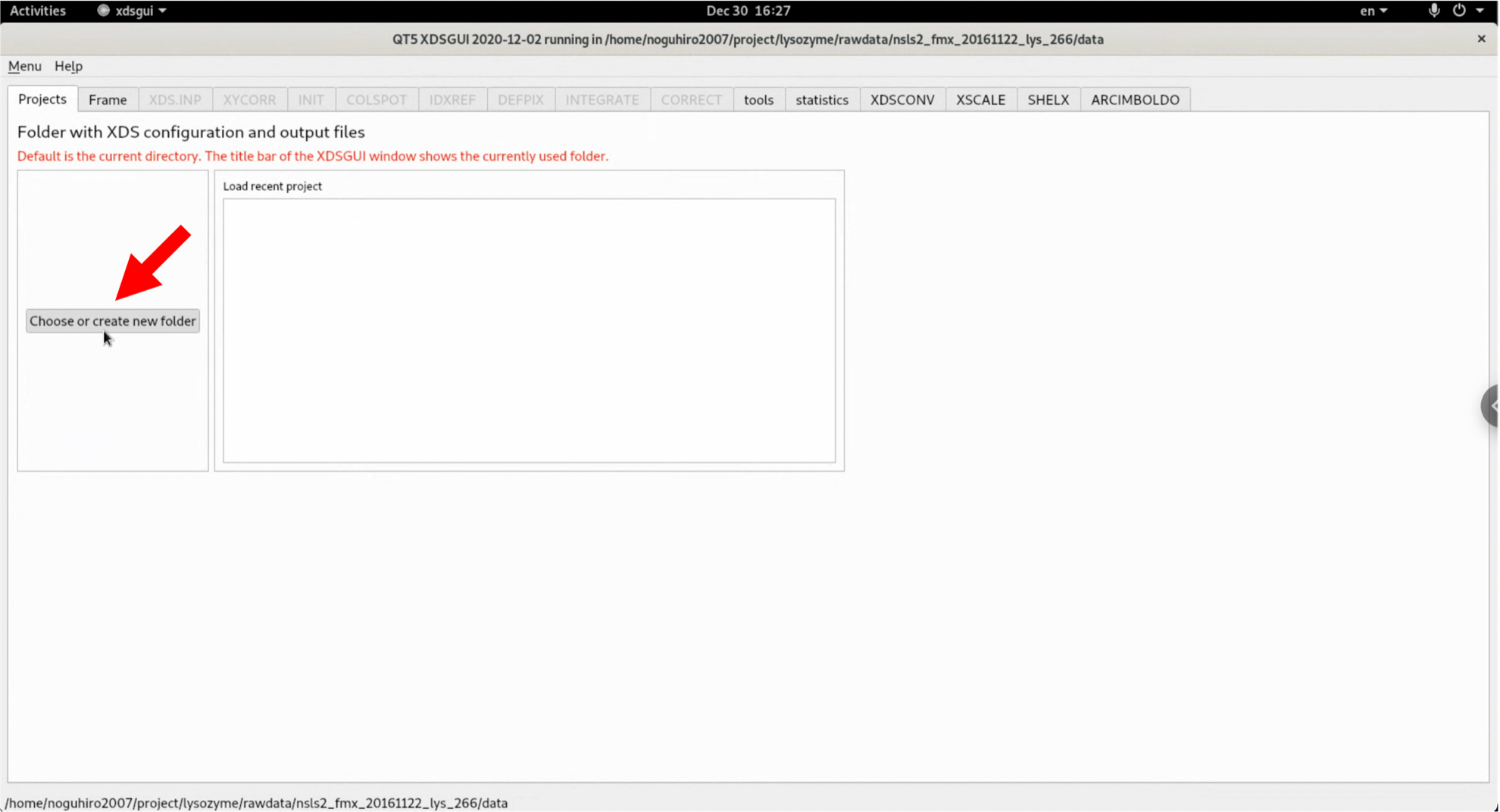
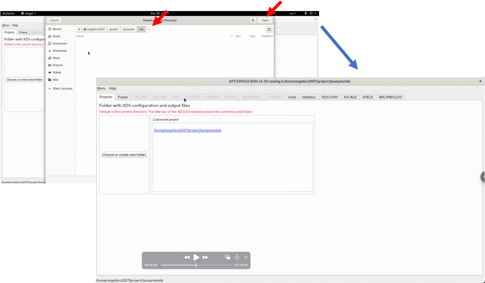
2. After launching xdsgui, select "Choose or create new folder" and designate the output folder (project folder) for files generated by XDS.
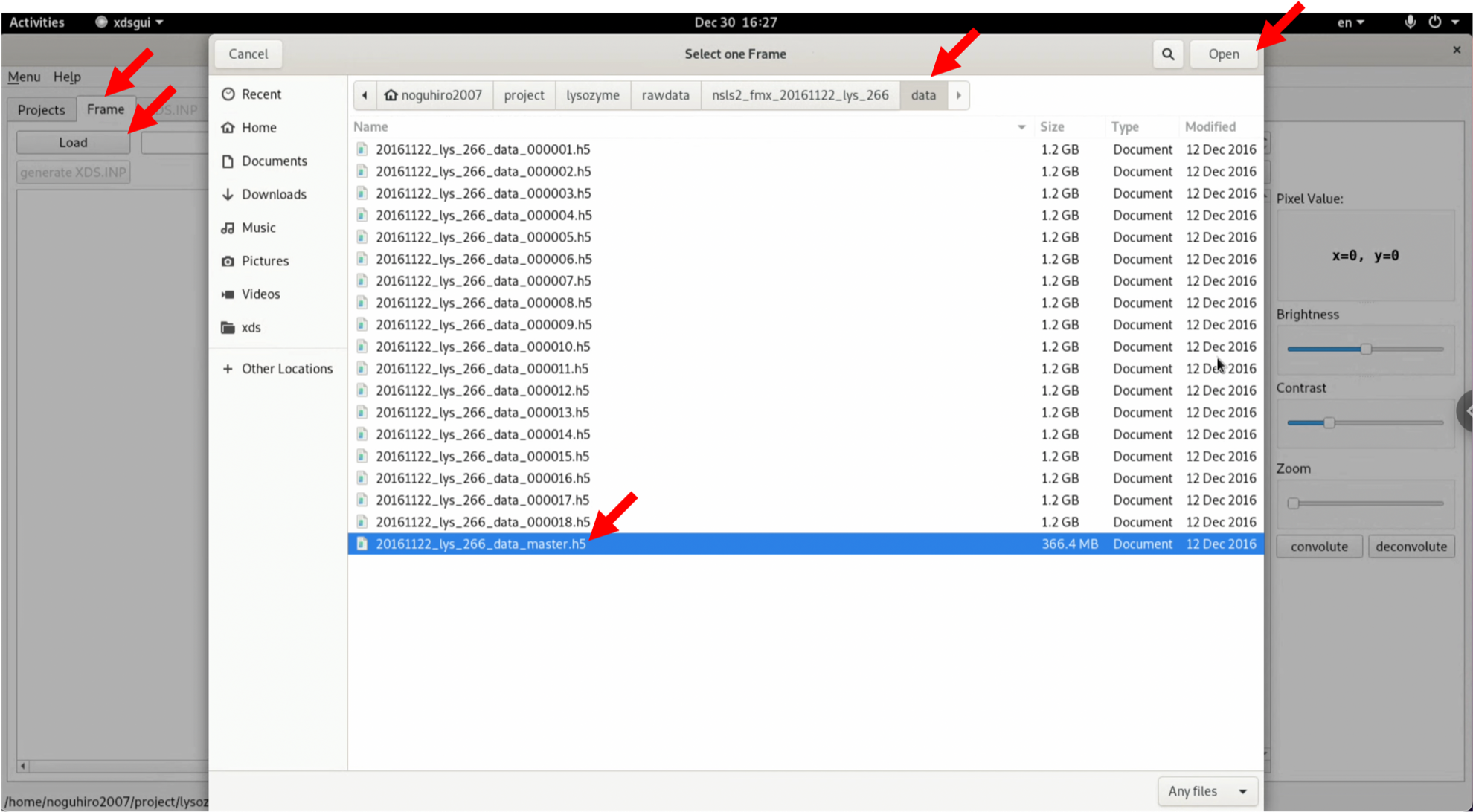
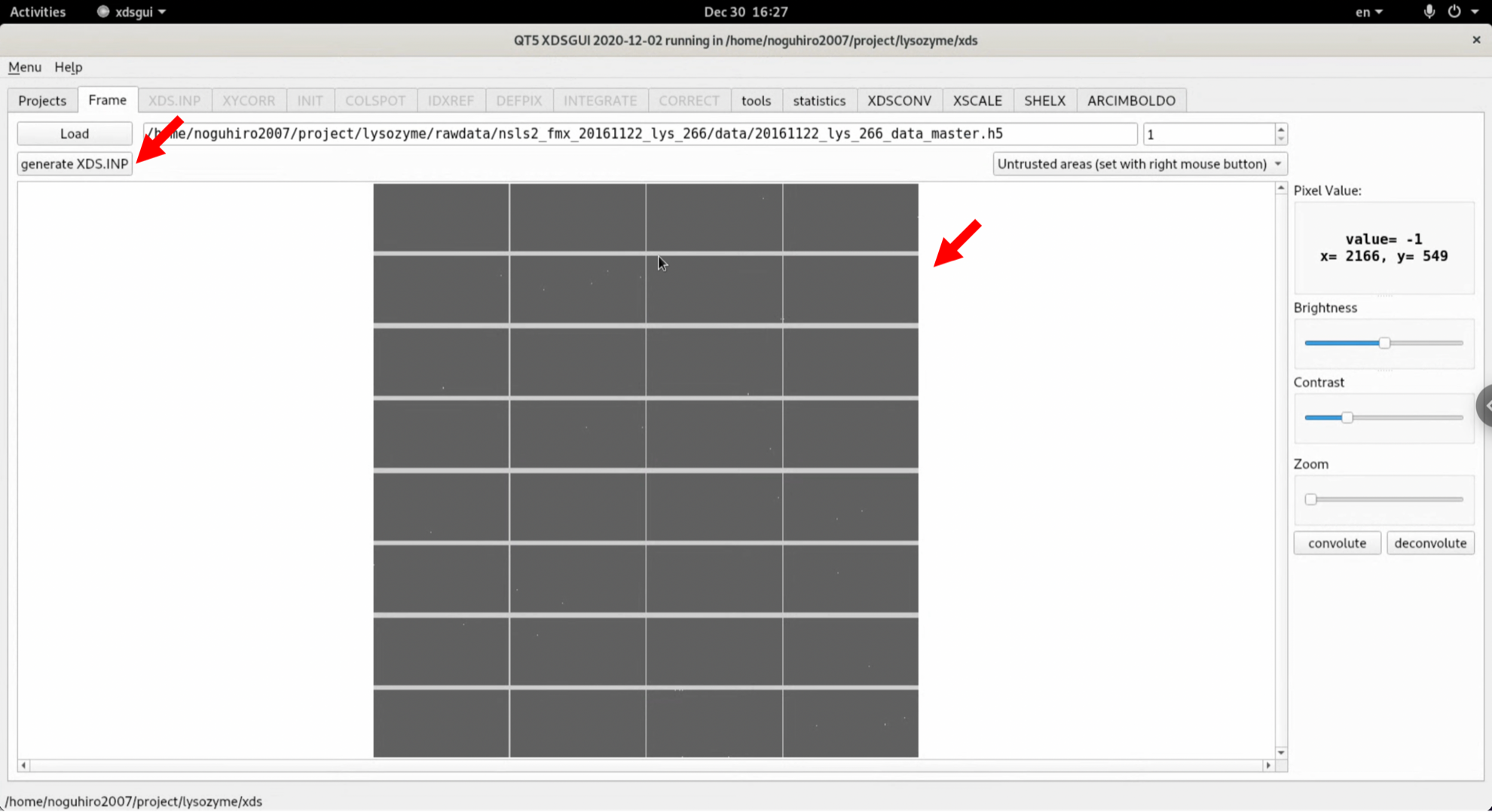
3. Click "Load" in the "Frame" tab, and from the diffraction image files that you have downloaded and unzipped, select "20161122_lys_266_data_master.h5" and open it. Be careful to specify the master.h5 file.
4. Confirm the displayed diffraction image. Currently, the No.0001 image is visible, but nothing is seen4. Click "generate XDS.INP" to automatically create XDS.INP, which describes the processing method of XDS.
5. Click the "XDS.INP" tab. The generated XDS.INP is displayed and editable. Try running it as it is, without editing the generated XDS.INP. If several favourable conditions are met, such as having immaculate data, the entire process can be completed in one shot even in this automatic state.
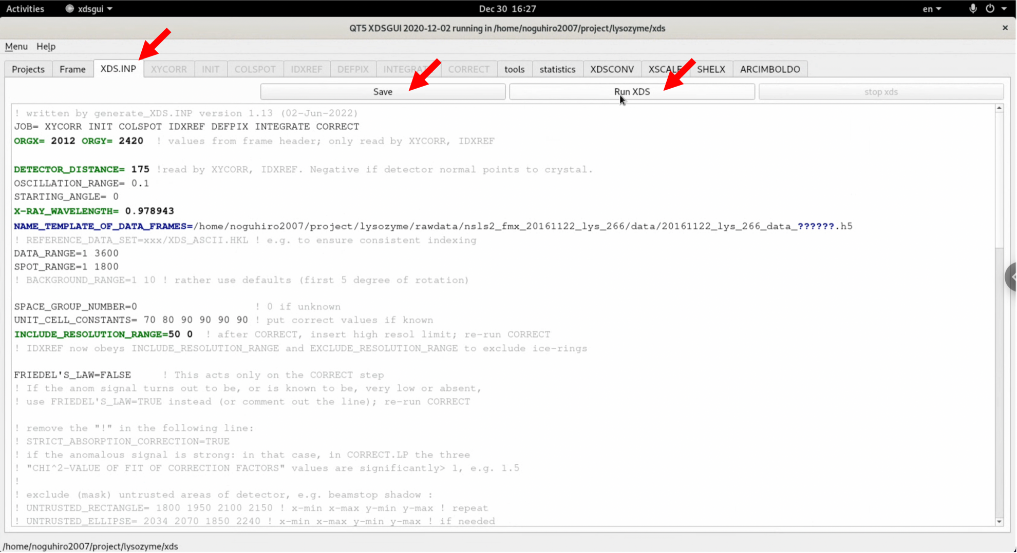
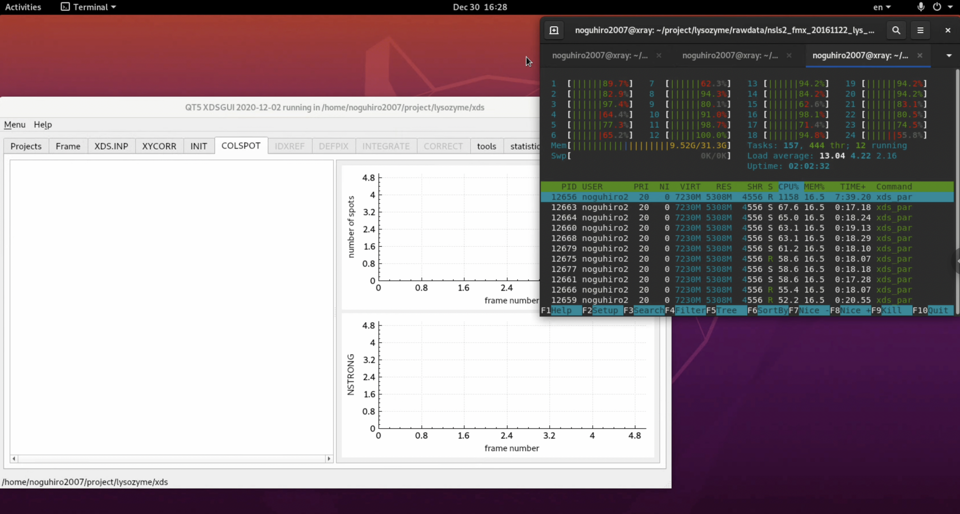
6. The process begins. During processing, nearly 100% of the CPU is used, so be careful when doing other work. Depending on the computing environment, you may have to wait several minutes.
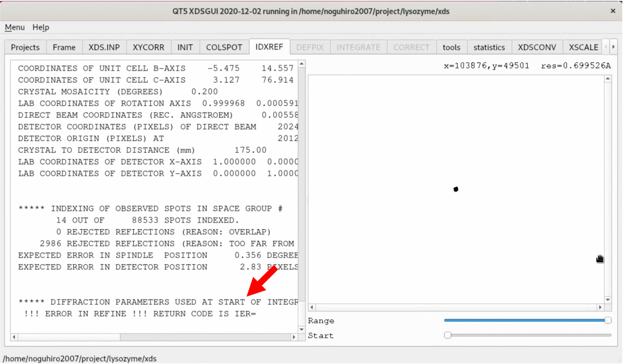
7. In the author's environment, an error occurred during the IDXREF step (Indexing). It appears that an error occurred during the parameter refinement process. As clearly shown in the diffraction image check, the first few images in this dataset do not have diffraction spots, which might be causing problems. Also, by default, 1,800 images (180°) are used for refinement, which is clearly excessive, so the range is narrowed.
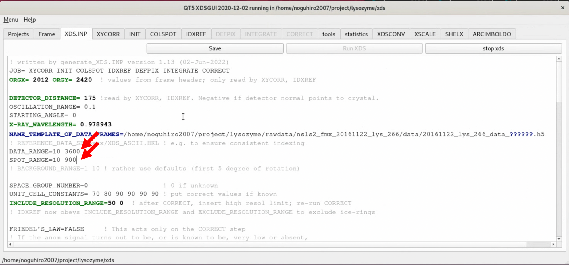
8. Open the XDS.INP editing screen from the "XDS.INP" tab, and change the following part. This will exclude the first 10 or so images, where no diffraction spots exist, from the process and limit the images used for the Indexing process to those up to 90° in rotation angle. After making the changes, start the process by clicking "Save" --> "Run XDS".
- DATA_RANGE=0 3600
+ DATA_RANGE=10 3600
- SPOT_RANGE=0 1800
+ SPOT_RANGE=10 900
(Scene of RunXDS)
In IDXREF, a Bravais lattice is predicted (Indexing) from the diffraction spots picked up by COLSPOT. Inside the software, it starts with the least probable Bravais lattice, aP (triclinic, $a\neq b \neq c$, $\alpha \neq \beta \neq \gamma$), and gradually fits more symmetric Bravais lattices, identifying the one with the highest symmetry that fits the picked-up diffraction spots. The most highly symmetric Bravais lattice chosen in this way is most likely the Bravais lattice of this crystal. In this case, it was predicted to be tP (simple tetragonal, $a = b \neq c$, $\alpha = \beta =\gamma =90°$) (refer to the following IDEXREF.LP).
...

*********** DETERMINATION OF LATTICE CHARACTER AND BRAVAIS LATTICE ***********

 The CHARACTER OF A LATTICE is defined by the metrical parameters of its
 reduced cell as described in the INTERNATIONAL TABLES FOR CRYSTALLOGRAPHY
 Volume A, p. 746 (KLUWER ACADEMIC PUBLISHERS, DORDRECHT/BOSTON/LONDON, 1989).
 Note that more than one lattice character may have the same BRAVAIS LATTICE.

 !!! WARNING !!! For unknown crystals an augmented lattice basis may have been
                 constructed that could obscure the recognition of the correct
                 unit cell. See: "merged subtrees" in this file (IDXREF.LP).

 A lattice character is marked "*" to indicate a lattice consistent with the
 observed locations of the diffraction spots. These marked lattices must have
 low values for the QUALITY OF FIT and their implicated UNIT CELL CONSTANTS
 should not violate the ideal values by more than
 MAXIMUM_ALLOWED_CELL_AXIS_RELATIVE_ERROR=  0.03
 MAXIMUM_ALLOWED_CELL_ANGLE_ERROR=           2.0 (Degrees)

  LATTICE-  BRAVAIS-   QUALITY  UNIT CELL CONSTANTS (ANGSTROEM & DEGREES)
 CHARACTER  LATTICE     OF FIT      a      b      c   alpha  beta gamma

 *  44        aP          0.0      37.2   78.3   78.5  90.1  90.0  90.0
 *  31        aP          0.2      37.2   78.3   78.5  89.9  90.0  90.0
 *  35        mP          0.4      78.3   37.2   78.5  90.0  90.1  90.0
 *  33        mP          2.5      37.2   78.3   78.5  90.1  90.0  90.0
 *  34        mP          2.5      37.2   78.5   78.3  90.1  90.0  90.0
 *  32        oP          2.7      37.2   78.3   78.5  90.1  90.0  90.0
 *  25        mC          7.5     110.8  111.0   37.2  90.0  90.0  89.9
 *  23        oC          7.9     110.8  111.0   37.2  90.0  90.0  89.9
 *  20        mC          8.1     111.0  110.8   37.2  90.0  90.0  90.1
 *  21        tP         10.2      78.3   78.5   37.2  90.0  90.0  90.1
    37        mC        249.9     161.3   37.2   78.3  90.0  90.1  76.7
    39        mC        250.1     161.1   37.2   78.5  90.0  90.1  76.6
    36        oC        252.2      37.2  161.3   78.3  89.9  90.0 103.3
    28        mC        252.3      37.2  161.3   78.3  89.9  90.0  76.7
    38        oC        252.3      37.2  161.1   78.5  89.9  90.0 103.4
    29        mC        252.4      37.2  161.1   78.5  89.9  90.0  76.6
    27        mC        500.1     161.1   37.2  110.8  90.0 133.4  76.6
    19        oI        507.6      37.2  110.8  117.0  89.9  71.4  90.0
    26        oF        622.9      37.2  161.1  161.3  86.9 103.3 103.4
    18        tI        630.3     110.8  117.0   37.2  71.4  90.0  90.1
     1        cF        999.0     116.9  116.9  117.0  95.9  95.7 142.9
     2        hR        999.0      86.8   86.9  117.0 118.0  62.1 100.7
     3        cP        999.0      37.2   78.3   78.5  90.1  90.0  90.0
     5        cI        999.0      86.9   86.7  110.8  50.4  50.3  79.5
     4        hR        999.0      86.8   86.9  116.9 118.0  62.1 100.6
     6        tI        999.0     110.8   86.9   86.7  79.5  50.4  50.3
     7        tI        999.0      86.9   86.7  110.8  50.4  50.3  79.5
     8        oI        999.0      86.7   86.9  110.8  50.3  50.4  79.5
     9        hR        999.0      37.2   86.8  250.8 102.6  98.5 115.4
    10        mC        999.0      86.7   86.8   78.5  90.0  90.1 129.2
    11        tP        999.0      37.2   78.3   78.5  90.1  90.0  90.0
    12        hP        999.0      37.2   78.3   78.5  90.1  90.0  90.0
    13        oC        999.0      86.7   86.8   78.5  90.0  90.1  50.8
    15        tI        999.0      37.2   78.3  179.3  64.1  78.0  90.0
    16        oF        999.0      86.7   86.8  179.3 107.7 118.9  50.8
    14        mC        999.0      86.7   86.8   78.5  90.0  90.1  50.8
    17        mC        999.0      86.8   86.7   86.9  79.5 100.7  50.8
    22        hP        999.0      78.3   78.5   37.2  90.0  90.0  90.1
    24        hR        999.0     179.1  111.0   37.2  90.0  78.0 108.0
    30        mC        999.0      78.3  175.4   37.2  90.0  90.0  63.5
    40        oC        999.0      78.3  175.4   37.2  90.0  90.0 116.5
    42        oI        999.0      37.2   78.3  179.3 115.9 102.0  90.0
    41        mC        999.0     175.4   78.3   37.2  90.0  90.0  63.5
    43        mI        999.0      86.7  179.3   78.3 115.9 154.6  61.1

 For protein crystals the possible space group numbers corresponding  to
 each Bravais-type are given below for your convenience. Note, that
 reflection integration is based only on orientation and metric of the
 lattice. It does not require knowledge of the correct space group!
 Thus, if no such information is provided by the user in XDS.INP,
 reflections are integrated assuming a triclinic reduced cell lattice;
 the space group is assigned automatically or by the user in the last
 step (CORRECT) when integrated intensities are available.


 ****** LATTICE SYMMETRY IMPLICATED BY SPACE GROUP SYMMETRY ******

BRAVAIS-            POSSIBLE SPACE-GROUPS FOR PROTEIN CRYSTALS
  TYPE                     [SPACE GROUP NUMBER,SYMBOL]
  aP      [1,P1]
  mP      [3,P2] [4,P2(1)]
 mC,mI    [5,C2]
  oP      [16,P222] [17,P222(1)] [18,P2(1)2(1)2] [19,P2(1)2(1)2(1)]
  oC      [21,C222] [20,C222(1)]
  oF      [22,F222]
  oI      [23,I222] [24,I2(1)2(1)2(1)]
  tP      [75,P4] [76,P4(1)] [77,P4(2)] [78,P4(3)] [89,P422] [90,P42(1)2]
          [91,P4(1)22] [92,P4(1)2(1)2] [93,P4(2)22] [94,P4(2)2(1)2]
          [95,P4(3)22] [96,P4(3)2(1)2]
  tI      [79,I4] [80,I4(1)] [97,I422] [98,I4(1)22]
  hP      [143,P3] [144,P3(1)] [145,P3(2)] [149,P312] [150,P321] [151,P3(1)12]
          [152,P3(1)21] [153,P3(2)12] [154,P3(2)21] [168,P6] [169,P6(1)]
          [170,P6(5)] [171,P6(2)] [172,P6(4)] [173,P6(3)] [177,P622]
          [178,P6(1)22] [179,P6(5)22] [180,P6(2)22] [181,P6(4)22] [182,P6(3)22]
  hR      [146,R3] [155,R32]
  cP      [195,P23] [198,P2(1)3] [207,P432] [208,P4(2)32] [212,P4(3)32]
          [213,P4(1)32]
  cF      [196,F23] [209,F432] [210,F4(1)32]
  cI      [197,I23] [199,I2(1)3] [211,I432] [214,I4(1)32]


 Maximum oscillation range to prevent angular overlap at high resolution limit
 assuming zero (!) mosaicity.
 Maximum oscillation range  High resolution limit
         (degrees)               (Angstrom)
              2.93                    4.00
              2.19                    3.00
              1.46                    2.00
              0.73                    1.00

 cpu time used                 47.0 sec
 elapsed wall-clock time        3.7 sec
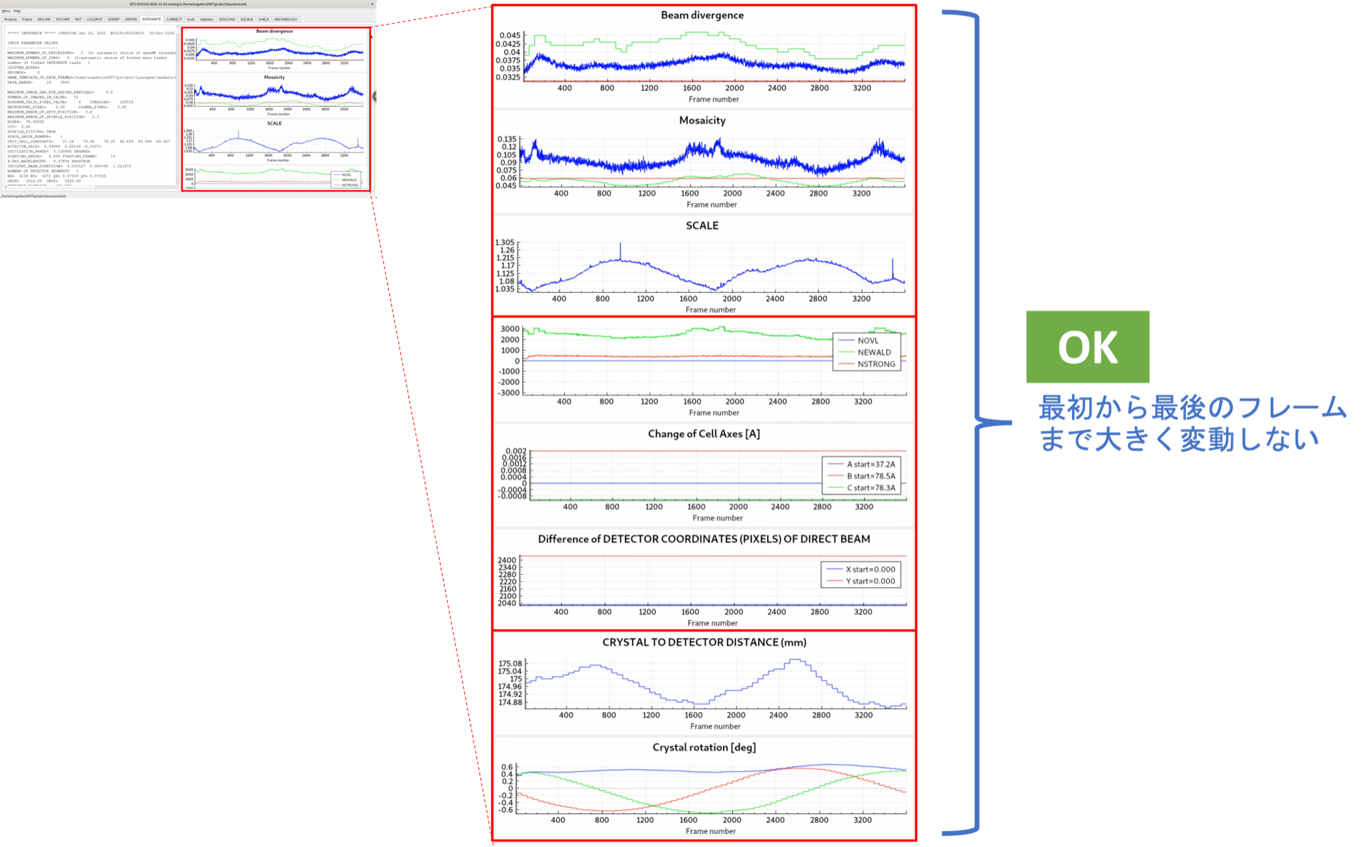
The parameters of the Bravais lattice estimated by IDXREF allow the software to predict where the diffraction spots of specific Miller indices $hkl$ (for example, $h=1, k=1, l=2$) should appear on the diffraction image. INTEGRATE collects the intensities of the diffraction spots within the specified diffraction image range (DATA_RANGE). On the right side of the INTEGRATE tab, graphed parameters for each frame during (and after) processing are displayed, enabling a broad overview of the dataset. Ideally, the graphs of each parameter should not fluctuate significantly. If there is a major deviation, it often indicates that the Bravais lattice estimated by IDXREF is incorrect.
The dataset used in this tutorial is of very high quality. It can serve as a positive control reference for future structure analysis.
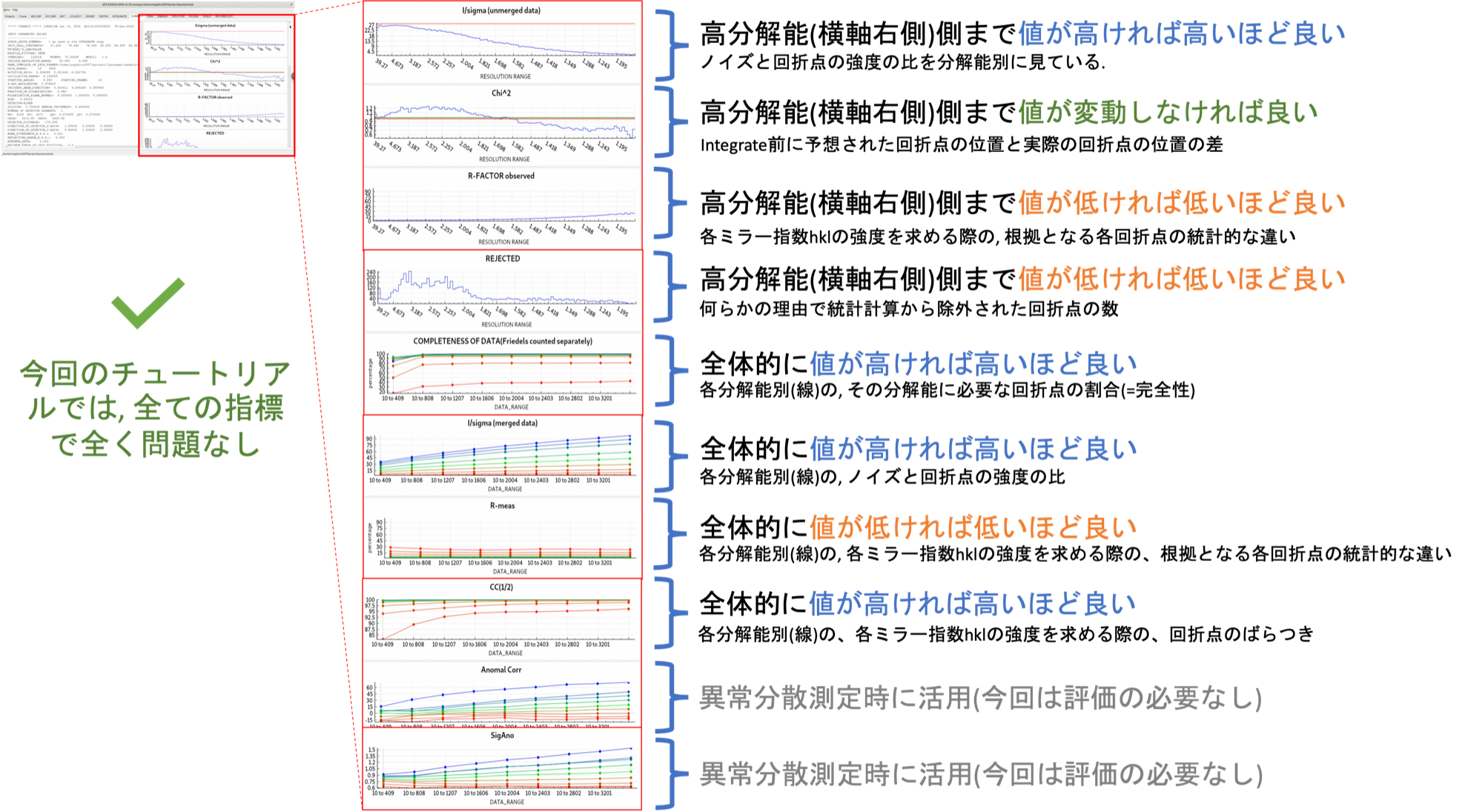
In the "COLLECT" tab, the software outputs statistically processed (Scaling) information, such as the intensities of each diffraction spot collected by INTEGRATE. On the right frame of the xdsgui, the results of the scaling are graphically displayed. A simplified explanatory diagram1 of various evaluation metrics is shown below. Please understand it as a basic concept. To reiterate, the dataset used in this tutorial has very clean statistical values and can serve as a positive control for your future reference.
Once the COLLECT step is successfully completed, you obtain the target file, XDS_ASCII.HKL. As the filename suggests, this text file contains not only the diffraction intensities and standard deviations for each $hkl$, but also information about crystallography.
!FORMAT=XDS_ASCII    MERGE=FALSE    FRIEDEL'S_LAW=FALSE
!OUTPUT_FILE=XDS_ASCII.HKL        DATE=30-Dec-2022
!Generated by CORRECT   (VERSION Jan 10, 2022  BUILT=20220820)
!PROFILE_FITTING= TRUE
!NAME_TEMPLATE_OF_DATA_FRAMES=/home/noguhiro2007/project/lysozyme/rawdata/nsls2_fmx_20161122_lys_266/data/20161122_lys_266_data_??????.h5 CBF
!DATA_RANGE=      10    3600
!ROTATION_AXIS=  0.999985  0.000941  0.005428
!OSCILLATION_RANGE=  0.100000
!STARTING_ANGLE=     0.000
!STARTING_FRAME=      10
!INCLUDE_RESOLUTION_RANGE=    50.000     1.152
!SPACE_GROUP_NUMBER=   89
!UNIT_CELL_CONSTANTS=    78.538    78.538    37.285  90.000  90.000  90.000
!UNIT_CELL_A-AXIS=     3.607    76.771    16.173
!UNIT_CELL_B-AXIS=     4.469   -16.365    76.684
!UNIT_CELL_C-AXIS=    37.185    -1.235    -2.431
!REFLECTING_RANGE_E.S.D.=     0.059
!BEAM_DIVERGENCE_E.S.D.=     0.031
!X-RAY_WAVELENGTH=  0.978943
!INCIDENT_BEAM_DIRECTION= -0.003116 -0.002702  0.999991
!FRACTION_OF_POLARIZATION=   0.980
!POLARIZATION_PLANE_NORMAL=  0.000000  1.000000  0.000000
!AIR=  0.000316
!SILICON=  3.700630
!SENSOR_THICKNESS=  0.450000
!DETECTOR=EIGER
!OVERLOAD=    125018
!NX=  4150  NY=  4371    QX=  0.075000  QY=  0.075000
!ORGX=   2032.29  ORGY=   2442.09
!DETECTOR_DISTANCE=   175.309
!DIRECTION_OF_DETECTOR_X-AXIS=   1.00000   0.00000   0.00000
!DIRECTION_OF_DETECTOR_Y-AXIS=   0.00000   1.00000   0.00000
!VARIANCE_MODEL=  1.621E+00  7.757E-04
!NUMBER_OF_ITEMS_IN_EACH_DATA_RECORD=12
!ITEM_H=1
!ITEM_K=2
!ITEM_L=3
!ITEM_IOBS=4
!ITEM_SIGMA(IOBS)=5
!ITEM_XD=6
!ITEM_YD=7
!ITEM_ZD=8
!ITEM_RLP=9
!ITEM_PEAK=10
!ITEM_CORR=11
!ITEM_PSI=12
!END_OF_HEADER
     0     0     1 -5.993E-03  3.902E-01  2086.1  2430.7   3080.7   0.00203 100 -11  -85.95
     0     0     2  5.995E-01  1.671E-01  2147.4  2426.4   3180.0   0.00388 100  18  -75.96
     0     0     2  7.318E-01  1.768E-01  2147.6  2444.7    955.6   0.00379 100  21   61.41
     0     0     3  1.334E+00  2.725E-01  2209.0  2423.4   3287.9   0.00532 100  20  -65.22
     0     0     3  6.267E-01  2.840E-01  2209.1  2448.1    848.0   0.00521 100  11   50.67

...

     1    63     4  2.772E+01  1.334E+01  2556.5     9.1   1034.2   0.73636  85  14  -60.96
    -1    63     4  2.473E+01  1.385E+01  2551.1     8.1   1015.7   0.73627  77  16  -60.42
     1    63     5  3.999E+01  1.502E+01  2648.6     9.4   1036.3   0.73959  87  20  -59.57
    -1    63     5  3.925E+01  1.509E+01  2643.2     8.1   1017.9   0.73959  78  18  -59.05
     1    63     6  7.619E+00  1.156E+01  2742.3     8.3   1039.1   0.74362  80  10  -58.13
     2    63     5  2.280E+01  1.282E+01  2650.6     8.2   1045.7   0.73984  78  13  -59.85
!END_OF_DATA
The author has uploaded the XDS processing results to Github.
Step.2-5-2 Determining Resolution and Format Conversion Using CCP4-AIMLESS
The output data from XDS, XDS_ASCII.HKL, is scaled and converted to the MTZ format used in subsequent steps. At the same time, the resolution of the structure factor $F(hkl)$ is determined. The AIMLESS log is described in a format that is very easy to handle when writing papers, so I often use AIMLESS. However, the same conversion can be done using XDSCONV from XDS.
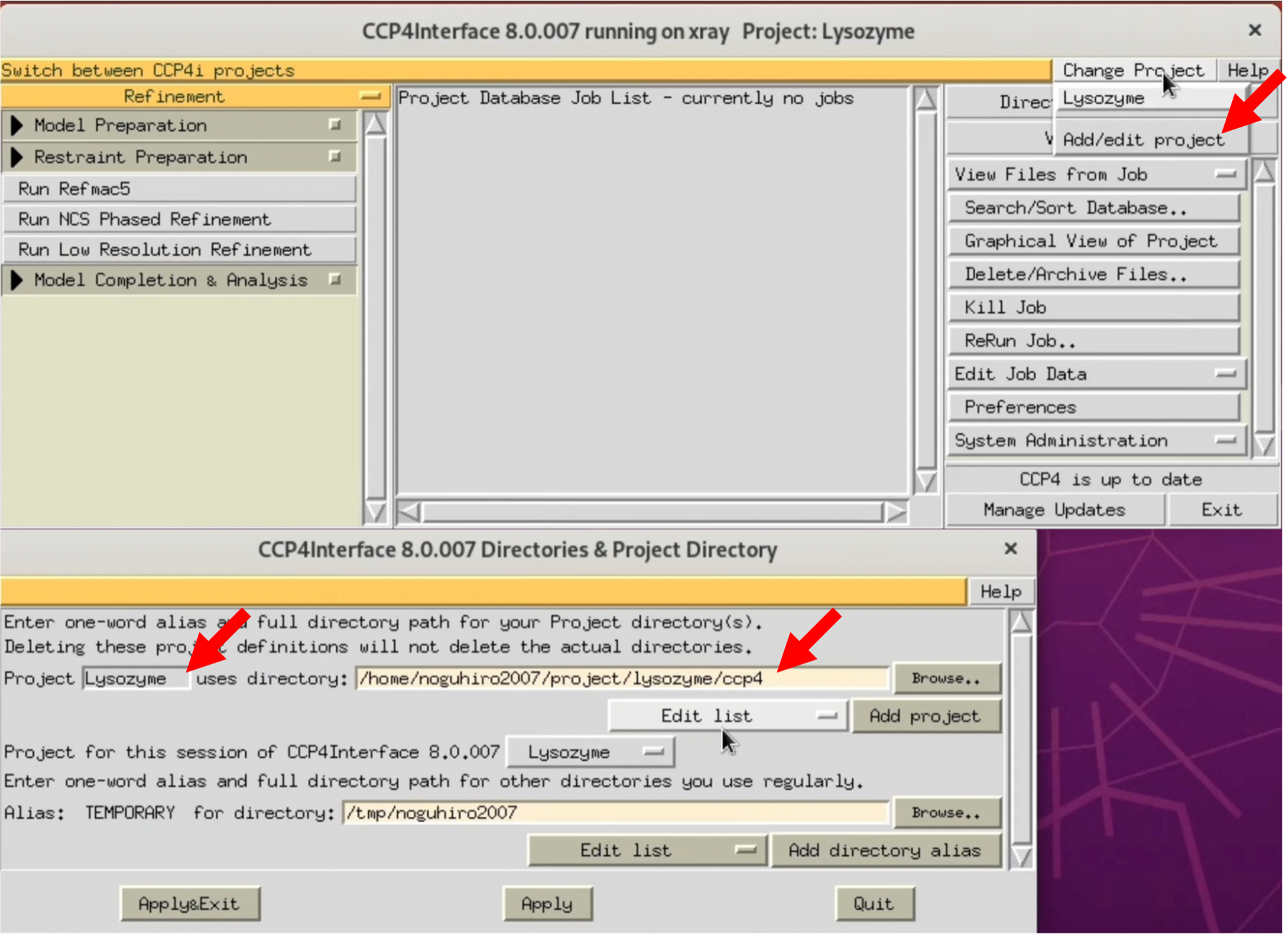
- Launch CCP4i and select the project used in this tutorial from "Change Project".
$ ccp4i
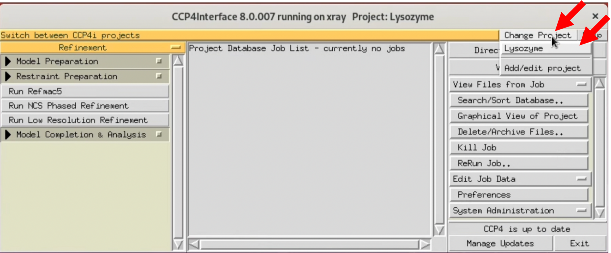
If you have not set up a project yet, create a new one from "Add/Edit project". Basically, all files output from CCP4 are saved in the Project folder. In this tutorial, the Project name was set to Lysozyme, and a specific folder for CCP4 was created and specified in the "uses directory".
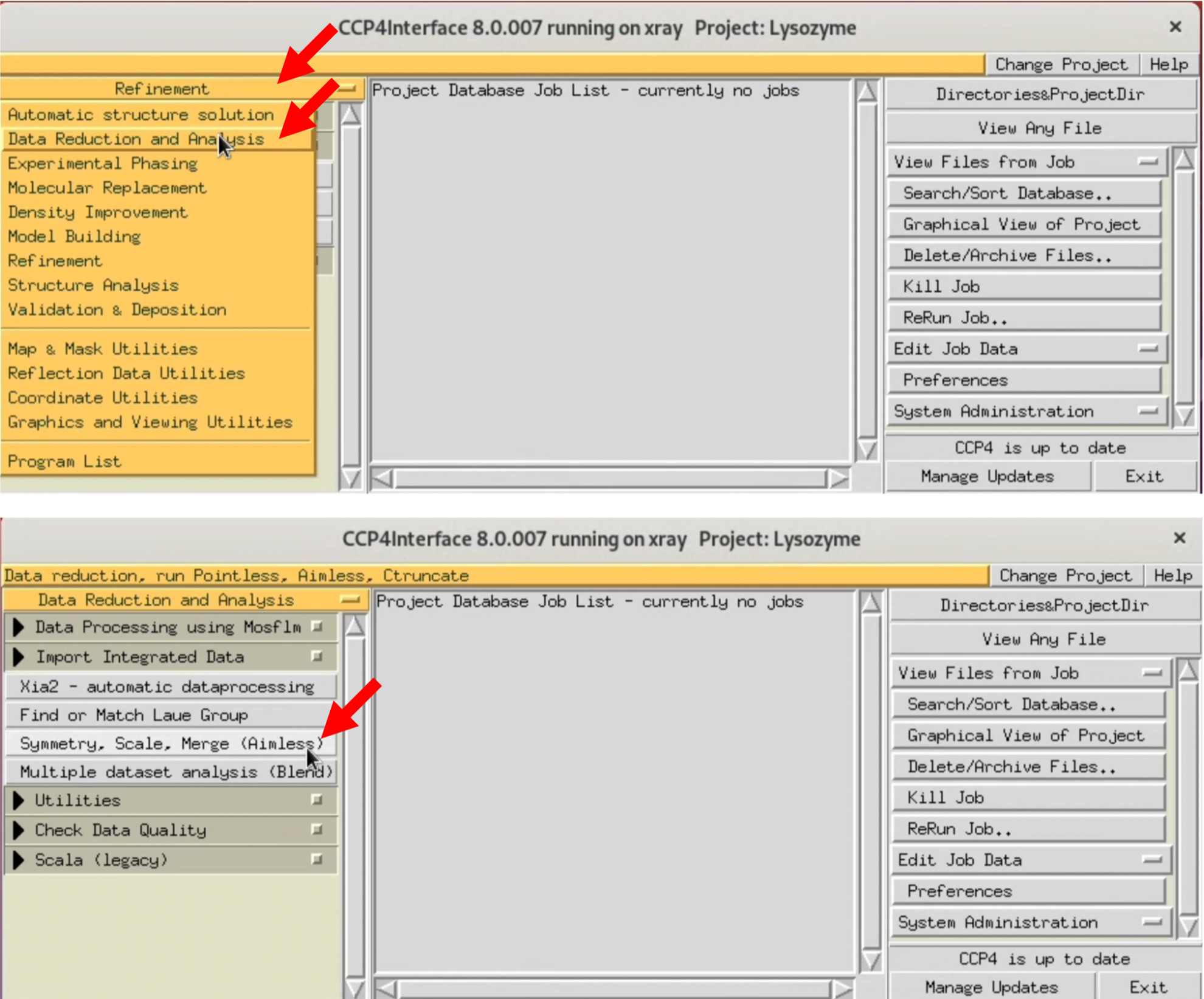
2. Select "Data Reduction and Analysis" from the left menu of CCP4i, and select Symmetry, Scale, Merge (Aimless) from the pop-up menu.
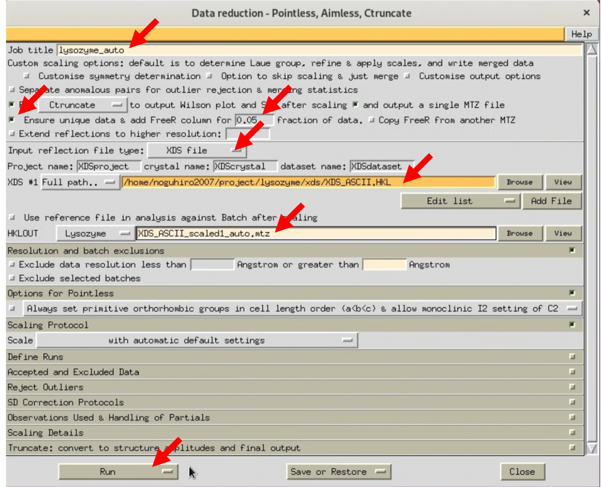
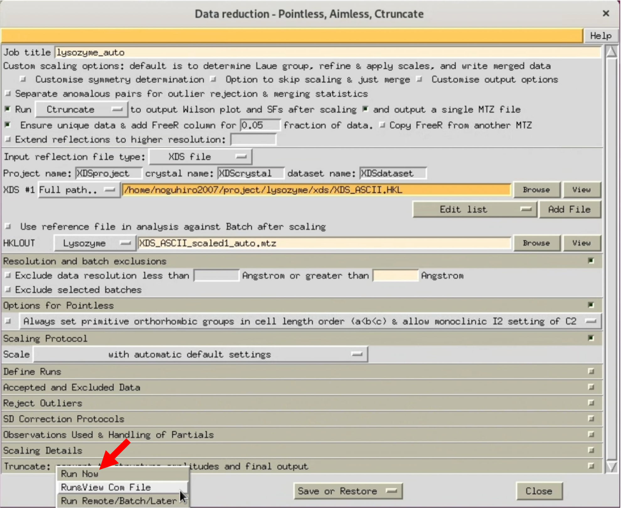
3. When the AIMESS Window opens, follow the red arrows in the image to set various settings. Start by not specifying the resolution, and process at the highest resolution to see how it goes.
The XDS processing results I performed are uploaded to Github. Please use it as needed.
While processing, the Status will be "Running", and when processing is finished, it will change to "FINISHED".
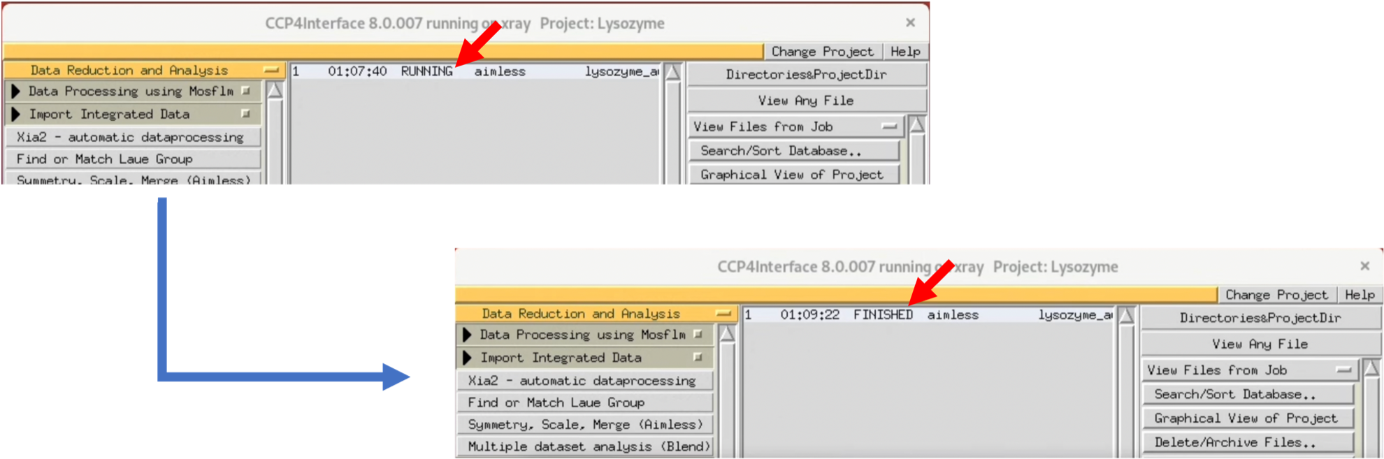
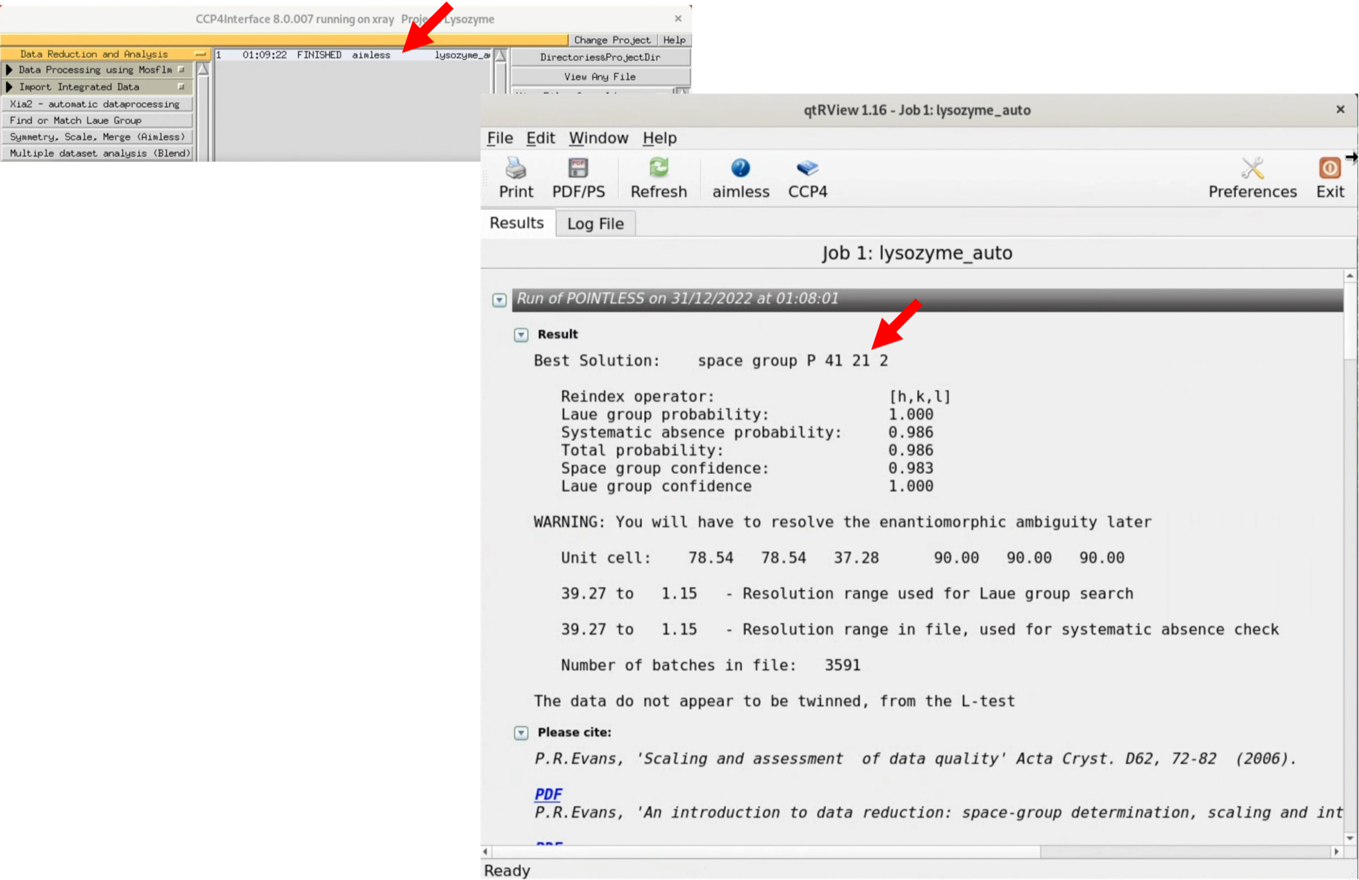
4. Once the Status changes to "FINISHED", you can view the graphical Log by double-clicking the Status item (the original is a text file). AIMLESS will automatically estimate the space group.
While the best solution is predicted to be the space group P41212, this space group is actually incorrect. However, in this tutorial, it's important to understand where we notice this mistake, so we'll continue on as if we don't know.
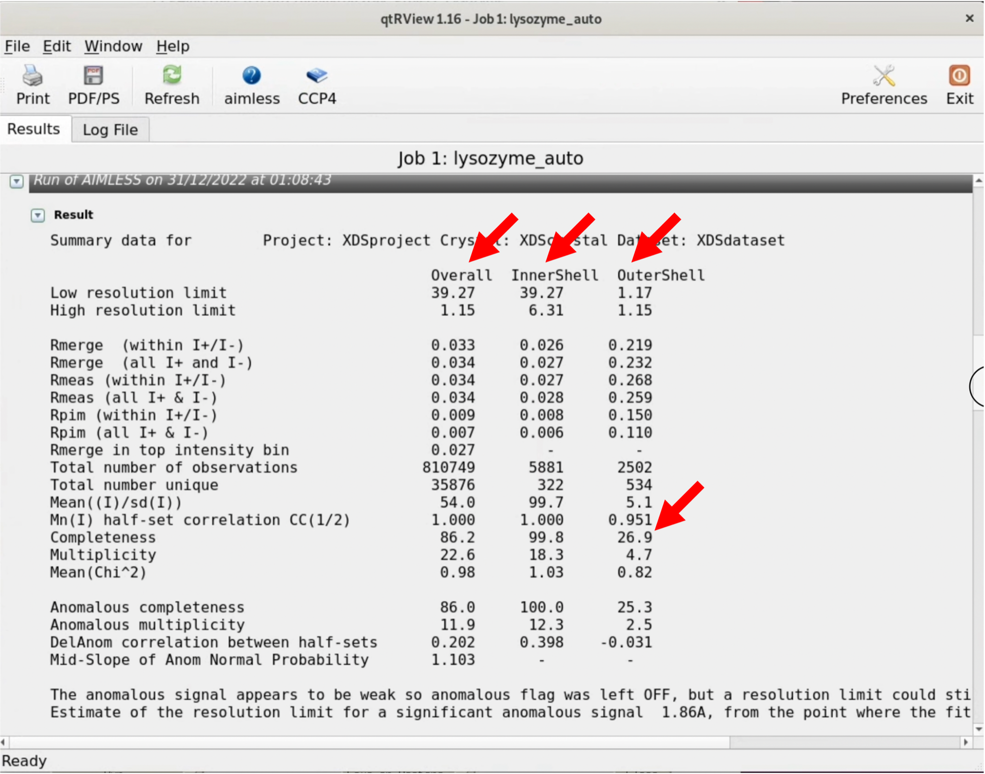
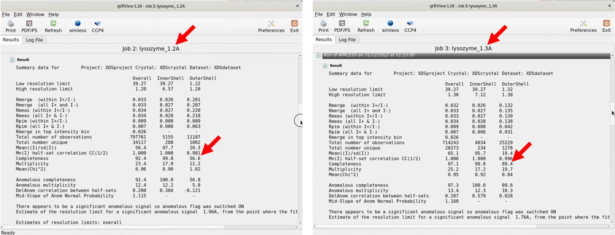
5. Scroll through the graphical log, and under "Run of AIMLESS on ~~", you'll see a very important table (see the image below). In this table, you can check the quality of the final structure factor $F(hkl)$ obtained from the diffraction image dataset. The resolution of the final dataset will be considered using the OuterShell column in particular. Below is a brief explanation of each item and an indicator for determining resolution.
There is ongoing debate about a universal indicator for determining resolution, and researchers have slightly different methods. The indicators in this table are meant as examples, assuming this background, and are thought to be safe.
| Item | Description | Range to include in the structure factor $F(hkl)$ (My opinion) |
|---|---|---|
| Rmerge | The difference between the structure factors that should be the same is divided by the measured structure factor. Defined by the following formula if there are N datasets. Generally expressed as a percentage %. A lower value indicates good reproducibility of the diffraction intensity experiment and indicates high-quality data. However, many problems have been pointed out, and its use as a quality judgment indicator is currently not recommended. 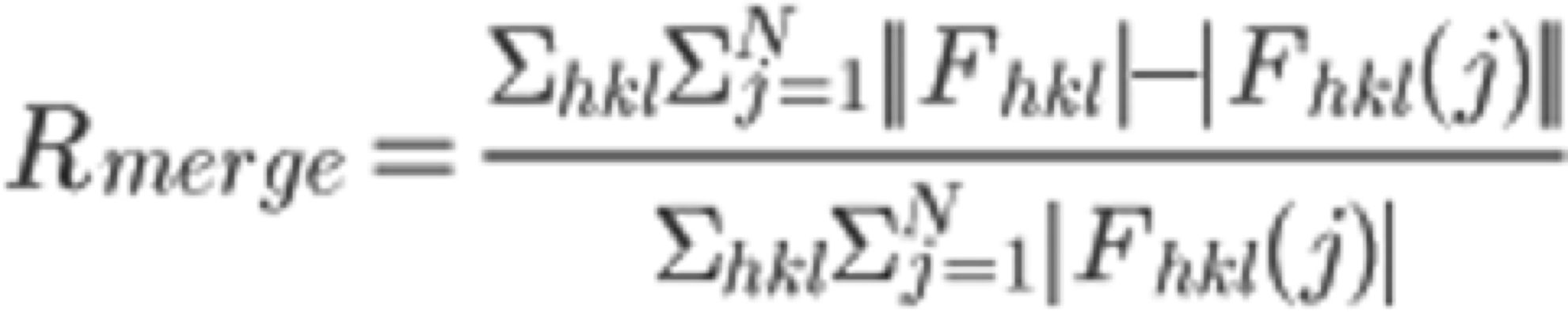
|
-- |
| Rmeas | Proposed as a replacement for Rmerge. It is an index for unmerged (individual) data that does not depend on multiplicity. Like Rmerge, the lower the value, the better the data. 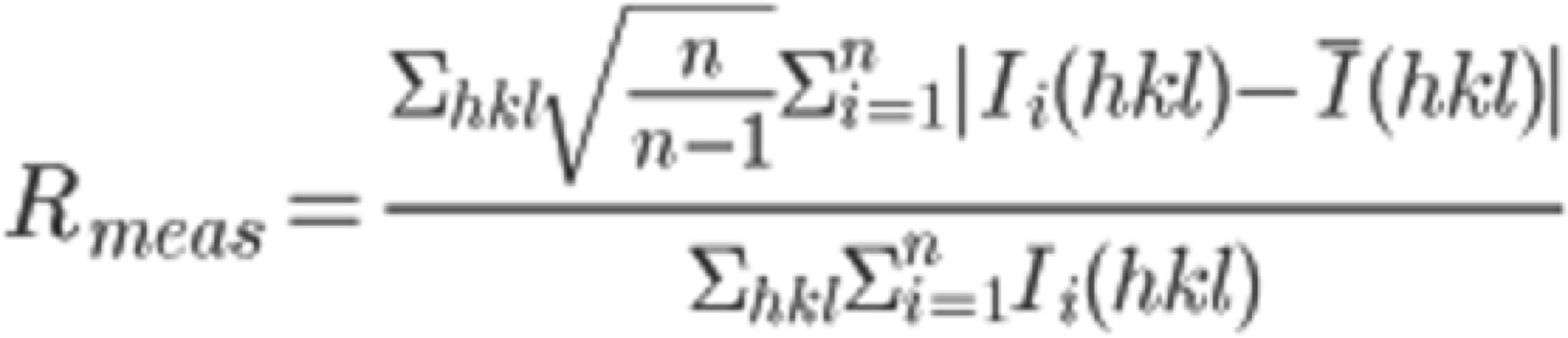
|
< 0.4 |
| Rpim | An R-value for merged intensities. The lower the value, the better the data. ![image.png] 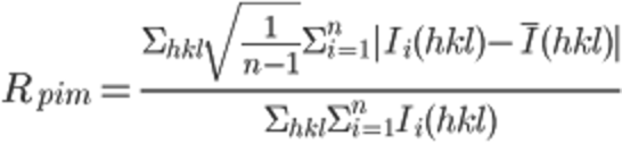
|
< 0.4 |
| Total number of observations | The total number of diffraction points where intensity has been integrated, recognized during the Integrate process. | -- |
| Total number unique | The number of diffraction points forming the mirror index $hkl$ of this dataset. Diffraction points with the same mirror index $hkl$ are statistically integrated. | -- |
| Mean ((I)/sd(I)) | The value obtained by dividing the average diffraction point intensity (I) by the average standard deviation of the measured values sd(I). A higher value implies a better S/N ratio, and increases the reliability of the diffraction point intensity. | > 2.0 |
| Mn(I) half-set correlation CC(1/2) | The half dataset correlation function. The observed values of each reflection are randomly divided into two, and the correlation coefficient between them is shown. It does not depend on $\sigma(I)$. CC(1/2)=1 indicates perfect correlation, and CC(1/2)=0 indicates no correlation. The calculation formula is shown below. $\sigma_y$ is the distribution of average intensities, and $\sigma_{\epsilon}$ is the averaged variance of merged intensities. 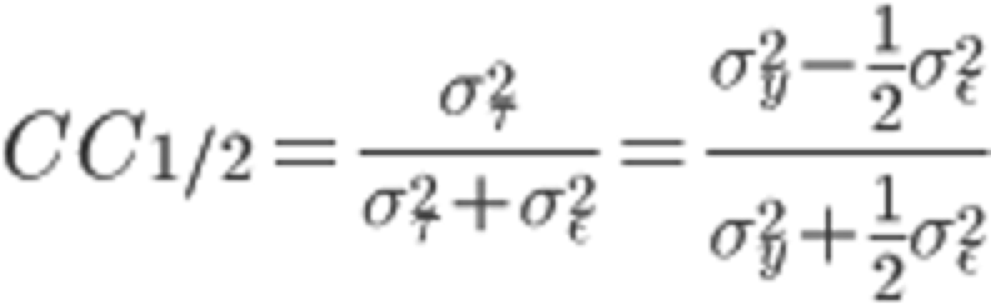
|
> 0.5 |
| Completeness | The value obtained by dividing the number of unique reflections obtained from measurements by the total number of unique reflections, represented as a percentage. | > 0.9 |
| Multiplicity | The value obtained by dividing the "Total number of observations" by the "Total number unique". A higher multiplicity value implies more diffraction points for each hkl intensity calculation, indicating a closer approximation to the true value. | > 1.0 |
| Mean(Chi^2) | -- | -- |
| Anomalous completeness | Not used in this tutorial. Completeness when $F^{+}$ and $F^{-}$ are captured separately, not the $F$ when the Friedel's law is valid. Important when dealing with anomalous dispersion. | -- |
| Anomalous multiplicity | Not used in this tutorial. Redundancy when $F^{+}$ and $F^{-}$ are captured separately, not the $F$ when the Friedel's law is valid. Important when dealing with anomalous dispersion. | -- |
| DelAnom correlation between half-sets | -- | -- |
| Mid-Slope of Anom Normal Probability | -- | -- |
Although the maximum resolution of the initial process is 1.15Å, the Completeness of OuterShell is too low at 26.9%, so we will lower the resolution, reconfigure, and perform Scaling again.
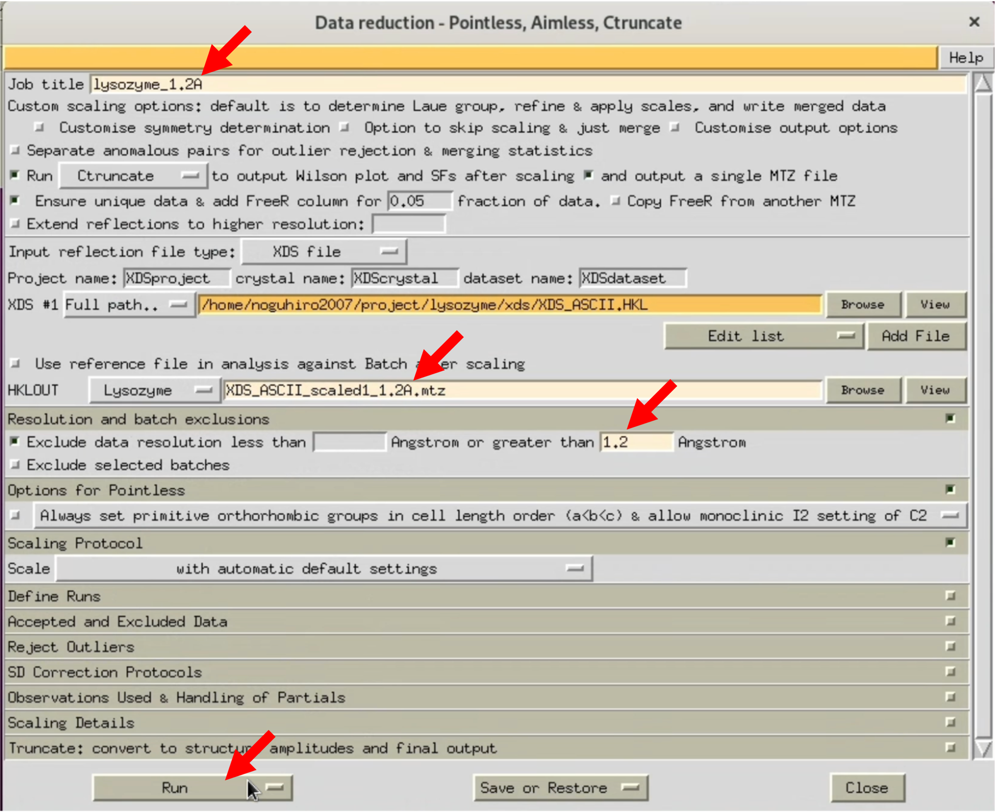
6. In the AIMLESS process setting window, under "Resolution and batch exclusions", enter the desired maximum resolution in the NNN part of "Exclude ~ greater than NNN Angstrom". This time, we will specify 1.20, 1.25, 1.30Å. At the same time, change the output file name (HKLOUT) and Job title accordingly. Perform a RUN with each resolution setting.
7. As a result, with a 1.3Å RUN, the Completeness of OuterShell becomes 89.4%, satisfying all conditions (some use the criteria of considering only resolutions where CC1/2 is above 0.5 as valid). Use the MTZ file outputted from the 1.3Å RUN, which in my case is XDS_ASCII_scaled1_1.3A.mtz, for Step.3.
8. That concludes Step.2. We will continue in Step.3(writing now) with the derivation of initial phases.
The results of the CCP4 AIMLESS processing conducted by the author areuploaded on GitHubした.
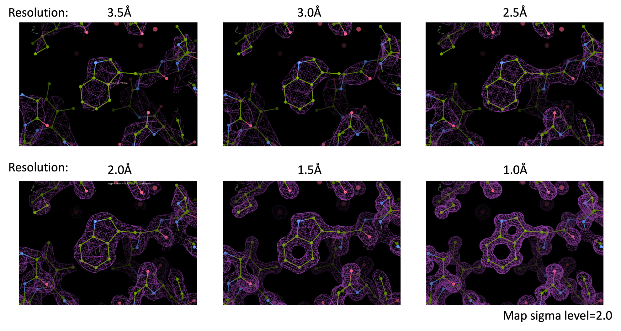
Step.2 Column: About Resolution
The word "resolution" has appeared in the text above, but it is very important in future analysis to have a sense of what kind of electron cloud you get with how much resolution. Therefore, below, I show electron cloud maps derived computationally for each resolution. At about 3.0Å resolution, almost all peptides can be traced and many side chains can be identified. Structural analysis can be easily done with a resolution of 2.5Å or higher. If a resolution of 1.5Å or higher can be obtained, almost every atom will be separated. In reality, many structures are analyzed at resolutions between 3.0Å ~ 1.5Å.
Conclusion
In this second edition of the Protein X-ray Crystal Structure Analysis Tutorial, we calculated diffraction images and structure factors $F(hkl)$. Using the obtained structure factor $F(hkl)$ file, we will determine the initial phase in the next step.
Table of Contents
- Step.0 The flow of structure determination
- Step.1 Installing analytical software
- Step.2 Checking diffraction images and calculating structure factors (this article)
- Step.3 Finding initial phases
- Step.4 Structure refinement and validation
-
Although it will be explained in Step 4, there are indicators to estimate the identity of the electron density map $\rho (xyz)$ and the protein model ($R$, $R_{free}$, etc.), and if these are too poor, it cannot be recognized as a reliable structure. ↩
-
The author once measured 130 crystal datasets in an 8-hour beam time. Assuming this pace is maintained for a full day, a staggering 1.404 million files would be generated, making file management extremely challenging for synchrotron or beamline managers if this goes on day after day. ↩ ↩2
-
A "good quality protein crystal" in layman's terms is "one where the protein is densely packed within the crystal, causing X-rays to diffract to high resolution." If the crystal is "small and heavy," the chances of this are high, but it could also be other low-molecular compounds in the crystal solution. If a large number of diffraction spots are confirmed at a resolution of 1.0~3.5Å, it can be determined to be a protein crystal. ↩
-
Probably the first few images were not exposed to X-rays due to some reason. This can cause problems with indexing, but in this tutorial, we will proceed as is. ↩