Protein X-ray Structure Determination Tutorial: Step.4 Structure Refinement and Validation

This article is written in English. Japanese Version is here.

Introduction

Welcome to the fourth instalment of our structural analysis tutorial series in the age of AlphaFold2 (First instalment, Second instalment, Third instalment). In this instalment, we'll refine the structure that we initially phased using AlphaFold2's predicted structure, to ultimately determine the X-ray crystal structure of Lysozyme.

Table of Contents

• Step.0 The flow of structure determination
• Step.1 Installing analytical software
• Step.2 Checking diffraction images and calculating structure factors
• Step.3 Finding initial phases
• Step.4 Structure refinement and validation (This article)

Target Audience and Purpose of This Article

This article aims to enable researchers, graduate students, and undergraduates who are not specialized in protein X-ray crystallography to understand the entire process of protein X-ray crystal structure analysis, from diffraction images to structure determination. We assume that readers have some familiarity with Bash commands in a Linux environment.

In this article, we will present a tutorial on protein structure analysis in a four-part series. This is the third part.

Also, this article is completely open. Whether at schools, research institutions, or companies, we would be delighted if you could spread this article and use it for educational purposes. However, we have not abandoned copyright.

Computing Environment Needed for Protein X-ray Crystallographic Analysis

From my experience, the following computing environment is suitable for protein X-ray crystallographic analysis. It requires computer power, so it's important not to attempt it on a Raspberry Pi or similar device.

• OS
  • Linux, such as Ubuntu, CentOS (strongly recommended)
  • MacOSX
  • Windows 10/11 (use either the native environment or a Linux environment on WSL2)
• CPU: > 4 cores (recommended: > 16 cores)
• Main Memory: > 16 GB (recommended: > 32 GB)
• Storage: > 50 GB (about 12 GB for software installation, data sets 20 - 30 GB/crystal)
• GPU: Not essential (recommended: equipped with a GPU)

In this step, we will perform the analysis on a virtual machine on Google Cloud Platform, which we set up inStep.1

Github Repository

Relevant files related to this tutorial are uploaded to Github. Feel free to refer to them as needed.
https://github.com/noguhiro2002/xray_tutorial

Step.4 Refinement and Validation of Structures

Step.4-0 Preparation

Step.4-0-1 What is Refinement and Validation?

The model structure of the protein Lysozyme obtained in Step 3, along with the initial phases, is merely a fit to the experimental data, using the structure "predicted" by AlphaFold2 as a rigid body. However, when observed at the amino acid level, there are spots where the structure does not match the experimental data. Therefore, in Step 4, we perform refinement and validation, fine-tuning the protein model structure to match the experimental data and ultimately achieving the final X-ray crystal structure of the protein. The process of structural refinement is as shown below. The model structure with initial phases obtained in Step 3 is first fit to the electron density cloud, ρ(xyz), using human judgment in ① COOT. Then, ② the refinement application Refmac is used to fit the structure factors, Fc(hkl) (the 'c' in Fc stands for 'calculated'), which are calculated from the model structure (coordinates and temperature factors B-factor of each atom), to the experimental structure factors Fo(hkl) (the 'o' in Fo stands for 'obtained'). This is done by refining the positions (xyz) and temperature factors (B-factor) of each atom in the model structure. The output model structure is then further tweaked in COOT, referencing the R-factor/R-free values, which indicate the level of agreement between Fc and Fo. This cycle is repeated several times, and finally, the model structure of the protein is confirmed to be free of problems in the quality check (validation) and to have the minimum R-factor/R-free values, thus determining the model structure of the protein.

Let's briefly explain the R-factor and R-free values, which are very important for structural refinement. The R-factor (also simply denoted as R) and R-free are essential values that indicate how well the model structure matches the experimentally obtained structure factors Fo(hkl) (the closer to 0, the higher the match), and they are calculated as follows.

\text{R-factor} = \frac{\sum ||Fo| - |Fc||}{\sum |Fo|}

However, there is a challenge in relying solely on the simple and convenient R-factor value for refinement (RCSB: Learn: Guide to Understanding PDB Data: R-value and R-free). For example, if all the electron clouds ρ(xyz) that should correspond to the protein are replaced with water molecule models, the R-factor value will be lower (= judged as numerically correct), resulting in a fundamentally incorrect structure. To solve this problem, the R-free indicator, which uses a method of cross-validation, is used. Specifically, about 5-10% of the structure factors Fo(hkl) are removed for verification, and the refinement is performed using the remaining approximately 95-90% of the data. After refinement, the R-value calculated using the excluded about 5-10% of the observed values is R-free. If a protein structure model that fits 100% to the electron cloud ρ(xyz) could be constructed (which is impossible in reality), the R-free value would be almost the same as the R-factor value. In reality, R-free takes a higher value than R-factor. Some researchers consider a value about 4% (0.04) higher than the R-factor to be just right.

Step 4-0-2: Strategy for Structural Refinement and Validation

Structural refinement is the process of deriving the atomic coordinates x,y,z and temperature factor B-factor of the model structure elements (such as protein molecules, water molecules, ligand molecules) that best fit the experimentally determined structure factors Fo(hkl). In this process, the initial phases α(hkl) are also optimized (see above Step.4-0-1). Let's take a look at the mmCIF file1 of Lysozyme registered in the actual PDB. The way the atomic coordinates x,y,z and temperature factor B-factor are shown in the mmCIF file is illustrated below. The protein structure of Lysozyme used in this tutorial alone has 1,001 atoms, each with four parameters (atomic positions x,y,z and temperature factor B-factor), bringing the total number of parameters to 4,004. The problem is that it is impossible to provide appropriate mathematical solutions to all these parameters with the amount of data for the structure factors Fo(hkl) obtained from the experiment¹.

Therefore, a strategy is needed to determine the atomic positions x,y,z and temperature factors B-factor that fit as closely as possible to the structure factors Fo(hkl) obtained experimentally. This is similar to the strategy used in numerical computation to find appropriate solutions, essentially starting from a small amount of input data and a small number of fitting parameters to find a rough solution, gradually shifting to a larger amount of input data and a larger number of fitting parameters to obtain a more detailed solution.

The concept is illustrated in the figure below. There's a risk that when fitting a large amount of input data (in this case, high-resolution data of experimentally obtained structure factors $Fo(hkl)$) to a large number of parameters all at once, a false solution that deviates from the most fitting value might be obtained as a local solution (shown as a blue dotted line when it fits the most, and as a black dotted line when a false value is obtained as a solution) (A). To avoid this, as shown in (B), a good strategy is to first approximate a solution using a small amount of input data and a small number of variables, and then gradually increase the quantity and number of both. This can avoid local solutions and smoothly obtain the optimal solution. This is an important strategy, especially in the refinement of high-resolution data structures exceeding 1.3Å, as in this case.

A question might arise here: "Even if a local solution like figure A is found, couldn't we tell it's the wrong solution by looking at the electron cloud $\rho (xyz)$? If so, why should we bother with a strategy like figure B?" This is a valid question, but it is hindered by a phenomenon called Phase Bias. The phenomenon of phase bias is illustrated in a paper titled "The Phase Problem" published in the scientific journal Acta Crystallographica Section D. The paper contains a useful figure that explains phase bias, which I am quoting below.

The Figure 3 of The phase problem. Garry Taylor, Acta Crystallographica Section D, Volume 59| Part 11| November 2003| Pages 1881-1890

This figure demonstrates a pseudo-structural factor data derived from a Fourier transformation of a picture of a duck, with phase information from a similar Fourier transformation of a picture of a cat mixed in, followed by an inverse Fourier transformation to recreate the image in real space. Normally, one might expect that adding the phase information of the cat's picture to the duck's picture would complicate the interpretation of the image. However, in reality, it is largely drawn to the phase information of the cat, and an image of the cat appears. This is the issue known as phase bias, where in actual structure refinement, you are drawn to the phase information of the wrongly placed structure, and a false electron cloud appears. As a result, those performing structure analysis may not notice this condition and output an incorrect model structure. This is not a unique phenomenon and is frequently observed during structure refinement, regardless of the overall structure or local structure. It is always necessary to be aware of phase bias when performing structure refinement.

Due to phase bias, a false electron cloud $\rho (xyz)$ may appear and even if it matches the model structure, the R-factor/R-free value is not affected and remains poor. Researchers can notice the error here, but by this point, the model structure fits well with the false electron cloud $\rho (xyz)$, and the position of the correct model structure becomes unclear. In other words, you are stuck in a local solution and it takes effort to recover.

Taking the above into consideration, I will outline the refinement process I performed on Lysozyme. This time, by repeating the structure refinement cycle shown above 11 times, I was able to determine the model structure. I will briefly describe each cycle below. Please use this tutorial as a reference for hands-on practice.

Cyc. No.	Comment
1	The entire protein structure obtained by molecular replacement (=AlphaFold2 structure) was treated as a rigid body (RBR, Rigid-Body Refinement) and the structure was refined at a resolution of 2.0Å. RBR is the most minimalist approach to refinement, seeking a very rough solution.
2	The resolution was kept at 2.0Å, and the refinement restraint method was changed from RBR to Restrained Refinement (see column below). This change increased the degree of freedom of each atom to move, greatly reducing the R-factor/R-free values, strongly confirming that the space group of this crystal was $P4_32_12$.
3	Continued refinement with Restrained Refinement and resolution. The R-factor/R-free decreased as with Cyc.2, but the rate of decrease slowed.
4	All other refinement parameters were maintained, but refinement was performed at the highest resolution of the data obtained this time (1.3Å). As a result, R-free improved considerably, but R-factor did not change much.
5	Here, the temperature factor parameter was changed from Isotropic to Anisotropic, significantly increasing the number of fitting parameters. This was necessary because the resolution of the structural factor $Fo(hkl)$ obtained was 1.3Å, and the number of parameters possessed by Anisotropic is necessary to represent the electron cloud $\rho (xyz)$ at this resolution. However, since the R-factor/R-free values did not decrease much, it was considered that the construction of the protein body model structure was almost finished.
6	Water molecules (structural water) existing around the protein model structure were added. As a result, the R-factor/R-free values dropped significantly.
7	Following the sixth round, the protein structure and structural water were modified. As a result, the R-factor/R-free values decreased significantly, as in the previous round.
8	From this cycle, the Ramachandran Plot and Geometry validation check tools of COOT were used to check the protein model structure.
9	Same as the 8th cycle. Only minor modifications were made.
10	Same as the 9th cycle. Only minor modifications were made. As the R-factor/R-free values settled down, it was considered that the construction of the protein body and structural water model was almost completed.
11	As a final touch, the model structure of Lysozyme was checked with MolProbity, and the model structure was corrected and refined, ultimately determining the model structure of Lysozyme.

Refmac5 Refinement Methods
As previously stated, one of the dilemmas in protein X-ray crystallographic analysis is the overabundance of parameters to be optimized (atomic positions $x, y, z$ and B-factors), compared to the input data. Therefore, limitations, based on known insights, are imposed on each optimization parameter, allowing for the construction of appropriate model structures. Notable examples include Ridig Body Refinement (RBR), Restrained Refinement, and TLS Refinement. Unrestrained Refinement, which does not consider any constraints, also exists, but unless there are conditions of high resolution (for example, above 1.0Å), it is impossible to obtain a reliable structure. The following briefly explains each representative refinement method.

• Rigid Body Refinement (RBR): Also known as rigid body refinement. Each subunit (per chain) of the model structure is regarded as a single rigid body, optimizing the six degrees of freedom (three translations and three rotations) that represent the position and orientation of the entire subunit. It is mainly used in the initial stage of structure refinement after obtaining initial phases using the MR method and is used to obtain a very rough solution.
• Simulated Annealing Refinement (SA): This is a method to avoid the model structure from falling into a local solution by pseudo-heating the structure model to high temperatures and gradually cooling it. While it was not implemented in this tutorial, it is advisable to conduct it after Ribid Body Refinement.
• Restrained Refinement: Considering the structural characteristics inherent in protein structures, revealed by ultra-high resolution structures of proteins reported so far and chemical constraints, this method performs refinement by reducing the actual number of parameters by adding binding conditions (stereochemical restraints: covalent bonds, angles, dihedrals, planarity, chirality, etc.) between atoms. At a resolution of about 1.3 - 3.0Å, which is usually obtained by protein structure refinement, structures are often determined by Restrained Refinement.
• TLS refinement: This method refines the B-factors of each atom by combining them with the rotation, translation, and vibration of the subunits (per chain) of the model structure. Considering the correlation of the B-factors of each atom, it can enhance the accuracy and reliability of the structural model. It is effective in cases of low resolution or particularly high B-factors of atoms (= the crystal has significant motion within the crystal). It is not a standard refinement method and is used when necessary.
• Unrestrained Refinement: As the name suggests, this refinement method maximizes the match between the observed structure factors $Fo(hkl)$ and the atomic coordinates ($x, y, z$) or B-factors without any constraints. It is the simplest, but ultra-high resolution (for example, above 1.0Å) is necessary, and there are not many applications in protein X-ray crystallographic analysis.

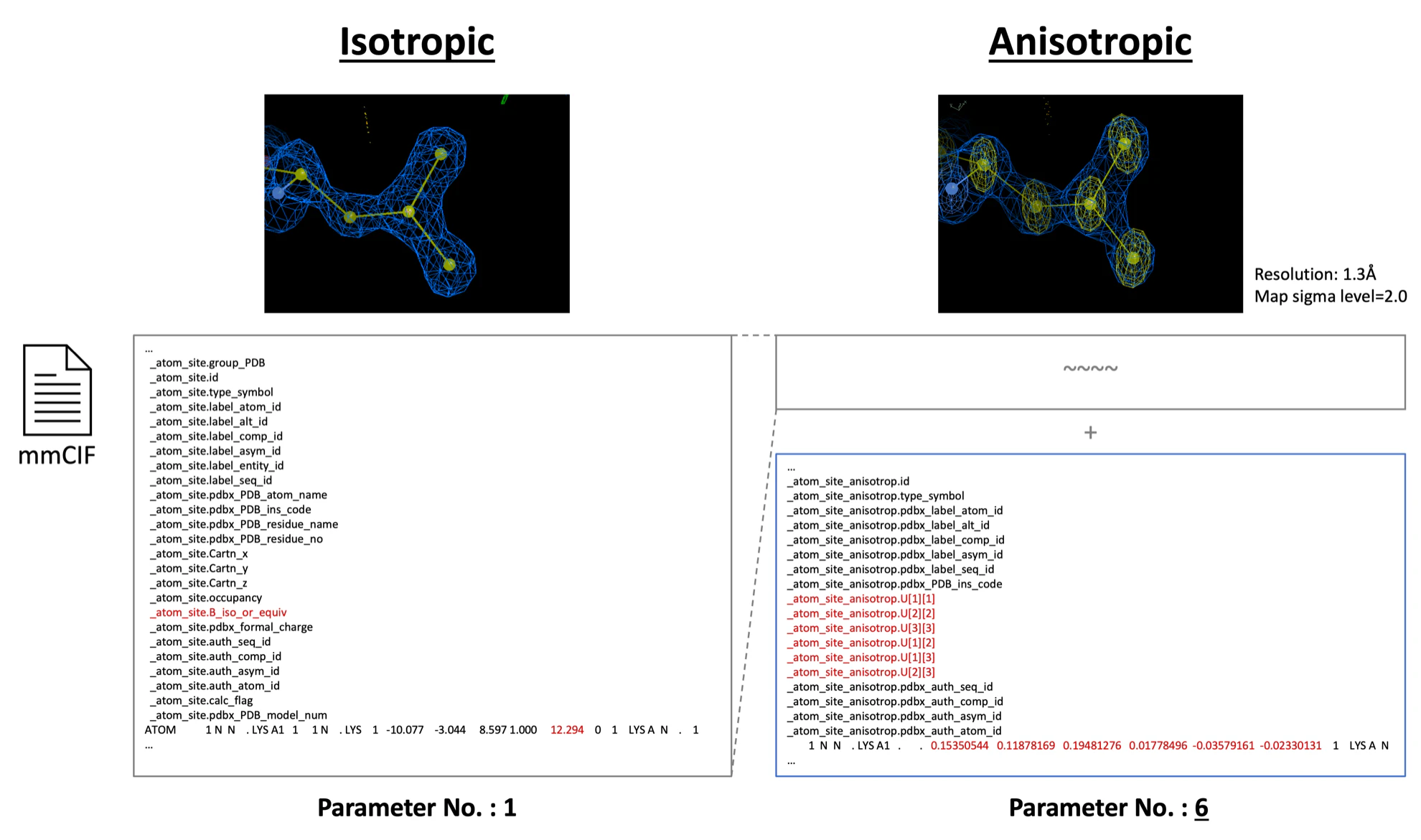
Isotropic vs Anisotropic
This refers to the different ways of expressing each atom's temperature factor (B-factor). Isotropic representation indicates the atom's temperature factor (B-factor) with a single value that doesn't depend on direction. Although scientifically, each atom's electron orbit is not circular, at the resolutions typically obtained in protein X-ray crystallographic analysis (about 1.3~3.0Å), it is impossible to observe the exact shape of each atom's electron cloud, and it is assumed to be spherical. On the other hand, at high resolutions of 1.3Å or more (the standard varies among researchers), due to the abundance of data, it is possible to represent the asymmetry and correlation of each atom's temperature factor (B-factor) more accurately, and it is expressed by six parameters (U-factors) that depend on direction. The image below shows how they are represented in actual mmCIF files. While Isotropic only has one temperature factor parameter (B-factor), Anisotropic records six temperature factor parameters (U-factors).

Types of Electron Density Maps $\rho (xyz)$
So far, we've referred to the electron density $\rho (xyz)$ in a simple manner, but in fact, there are mainly two types of electron density maps used in X-ray crystallographic analysis of proteins: the 2Fo-Fc map and the Fo-Fc map, which are commonly referred to as "electron cloud $\rho (xyz)$". In COOT, as shown in figure A below, the 2Fo-Fc map is indicated by a blue map, and the Fo-Fc map is indicated in green/red (green represents positive density, and red represents negative density). During structural refinement, these two maps are utilized appropriately at crucial points.

In the case of Figure A below, the orientation of the amino acid side chain is present in the negative Fo-Fc map, indicating that this orientation does not match the experimental data. Therefore, it is corrected to match the positive map of Fo-Fc, as shown in Figure B.

Below, the two maps are briefly explained:

• 2Fo-Fc Map : This map is calculated by doubling the structure factor $Fo(hkl)$ obtained from the experiment, then subtracting the structure factor $Fc(hkl)$ calculated from the model structure, resulting in the 2Fo-Fc map. As is evident from the calculation formula, if the model is properly placed, a normal-density electron cloud map will appear, but if the model is not placed there, a highlighted electron cloud map will appear.
• Fo-Fc Map : This map is calculated by simply subtracting the structure factor $Fc(hkl)$ calculated from the model structure from the structure factor $Fo(hkl)$ obtained from the experiment, resulting in the Fo-Fc map. When Fo > Fc, it is called a positive density map (where Fo-Fc is a positive value), indicating "there is something there" (displayed in green by default in COOT). When Fo < Fc, it is called a negative density map (where Fo-Fc is a negative value), indicating "placing the model structure there is a mistake" (displayed in red by default in COOT).

Step 4-1 Structure Refinement

Let's carry out actual structure refinement. As a preparation, I will explain a simple way to use COOT, which we use for modifying the model structure, and the concept of the asymmetric unit (ASU).

Step 4-1-0 COOT Operation Method and Asymmetric Unit (ASU)

Step 4-1-0-1 COOT Operation Method

Below are instructions on how to operate COOT. These are fundamental operations, so please try them all before proceeding with the refinement. Please note that a mouse, rather than a touchpad, is recommended as the third button of the mouse will be fully utilized.

Action	Operation	COOT's movement
Rotation	Left-click
Parallel translation (xy axis)	or Ctrl + Left-drag/Third-button drag
Zoom	Right-drag (Up/Down)
Prallel translation (z-axis)	Ctrl + Right-drag (Up/Down)
Move to Next Amino Acid/Water/Ligand	Space
Move to Specific Atom	第3ボタン (原子選択)
Electron Cloud Map (Depth)	Ctrl + Right-drag (Left/Right)
Change Contour Level of Electron Cloud Map	Scroll Wheel

Step.4-1-0-2 Understanding the Asymmetric Unit (ASU)

When visualizing protein molecules using Coot, what is shown is the Asymmetric Unit (ASU). Not limited to protein structures, "crystals" are formed by molecules arranged and overlapping in specific patterns. The minimal unit that can represent this crystal is the Asymmetric Unit (ASU). To explain it simply, the Unit Cell, the structural unit of the crystal, is formed by the Asymmetric Unit (ASU). These Unit Cells fill the space regularly, forming a crystal.

A noteworthy point is the fact that "Asymmetric Unit (ASU) ≠ Biological Unit". That is, the protein structure displayed in Coot does not necessarily represent the molecule's functional state in its natural environment. For instance, the haemoglobin protein (Woolly Mammoth Hemoglobin) that carried oxygen in the massive body of the woolly mammoth, which went extinct about 12,000 years ago, functions as a Biological Unit comprising two α-proteins and two β-proteins, a total of four proteins. However, the structure registered in the PDB (technically the R structure, 3VRF), consists of an Asymmetric Unit (ASU) formed by one α-protein and one β-protein.
The size of the Asymmetric Unit (ASU) can differ based on the crystal itself. Indeed, in a different structure of the aforementioned Woolly Mammoth Hemoglobin (technically the T structure, 3VRE), the Asymmetric Unit (ASU) and the Biological Unit coincide.

Please visit each linked site for more details and to compare the structures registered in the PDB and the Biological Units.

Step.4-1-1 Cycle.1

Parameter	Value
Refinement method	RBR
Resolution	2.0Å
B-factor	Isotropic
Target	Protein Structure

Actually, the first cycle of refinement was already carried out in the previous Step.3-2-4, using MR method with Structure Factor F(hkl) (Space Group: P43212). The first cycle of refinement often takes place to validate the MR method.

As seen in the video, the refinement (and the MR method) is working well.

Step.4-1-2 Cycle.2

Parameter	Value
Refinement method	Restrained Refinement
Resolution	2.0Å
B-factor	Isotropic
Target	Protein Structure

After refining with RBR, all the amino acid residues in the protein structure are checked, mainly for whether the backbone/side chains are not deviating from the electron cloud $\rho (xyz)$. In this tutorial, we used AlphaFold2 to accurately predict a classic structure, Lysozyme, and fitted it to very high-quality structure factors $F(hkl)$. So, we judged (and actually did) that it broadly matched at the RBR stage and performed Restrained Refinement once before structural correction with COOT (those without expert knowledge should perform the content of the next Cycle.3 here).

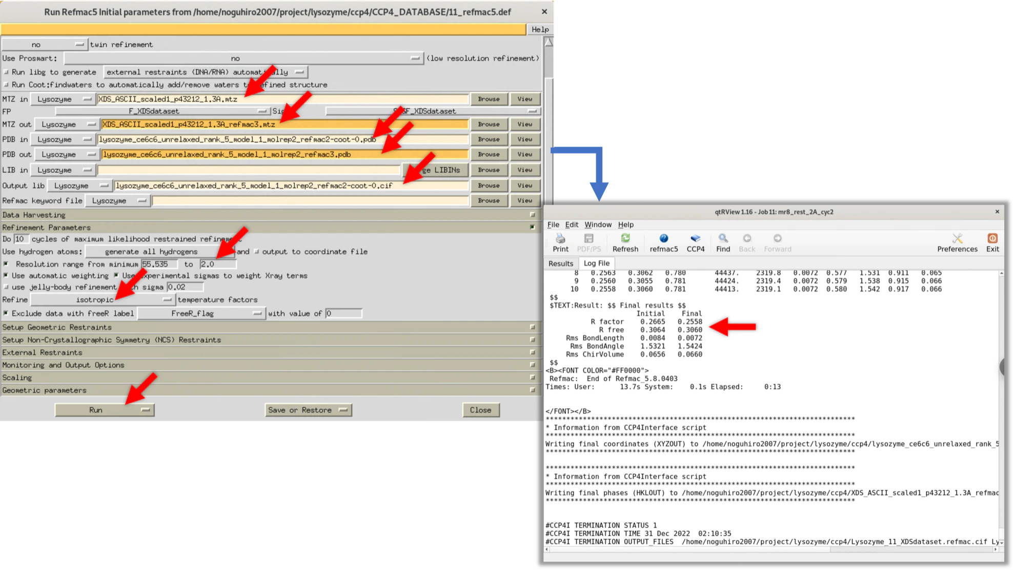
We will provide the setting values of Refmac and the logs at the time of execution (values at the time of the author's implementation. There is no problem if the values are about the same).

Step.4-1-3 Cycle.3

Parameter	Value
Refinement method	Restrained Refinement
Resolution	2.0Å
B-factor	Isotropic
Target	Protein Structure

Having improved the electron cloud $\rho(xyz)$ in Cycle.2, we now manually adjust the structure. The video below (5 times speed) shows this process. In this way, we carefully check and improve each residue from the N-terminus to the C-terminus of the protein chain. If there are parts where the main chain and side chains do not match the electron cloud map (both 2Fo-Fc and Fo-Fc maps), we adjust those parts using Real Space Fitting. If a large region does not match between the electron cloud map and the model structure, it may be more effective to first delete the model structure (the trash can icon on the right side of COOT has the delete function), then build a new protein backbone structure (the icon on the right side of COOT with one residue of amino acid marked on the + sign has the add function).

Again, we will provide the setting values of Refmac and the logs at the time of execution (values at the time of the author's implementation. There is no problem if the values are about the same).

Step.4-1-4 Cycle.4

Parameter	Value
Refinement method	Restrained Refinement
Resolution	1.3Å
B-factor	Isotropic
Target	Protein Structure

We review the areas adjusted in Cycle.3 and make further corrections where the electron cloud map still doesn't match. When the author performed this, the match between the electron cloud and the model structure of Lysozyme was high at this point, so the structure factor $Fo(hkl)$ with a resolution of 1.3Å was used for Refmac execution. As a result, R-factor/R-free became 0.258/0.271, and R-free significantly dropped.

Again, we will provide the setting values of Refmac and the logs at the time of execution (values at the time of the author's implementation. There is no problem if the values are about the same).

Step.4-1-5 Cycle.5

Parameter	Value
Refinement method	Restrained Refinement
Resolution	1.3Å
B-factor	Anisotropic
Target	Protein Structure

Just as when the resolution was 2.0Å, we have now adjusted the protein model structure to fit the 1.3Å electron density map in COOT. By this stage, there is almost complete alignment, including side chains. Thus, we have determined that the refinement using isotropic is largely completed, and have now performed anisotropic refinement, which is possible because the resolution is 1.3Å. As a result, the R-factor/R-free values have slightly decreased, indicating that the fitting has been improved due to the parameter increase by anisotropic. However, since the drop was small, it was considered that the refinement of the main body of the protein has almost finished.

For actual structural modifications using COOT, please refer to the video below (5x speed).

We also provide the settings and the log of Refmac during execution (based on the author's settings. Similar values should be fine).

Step.4-1-6 Cycle.6

Parameter	Value
Refinement method	Restrained Refinement
Resolution	1.3Å
B-factor	Anisotropic
Target	Protein Structure + Water

We have added water molecules (structural water) that exist around the protein model structure. These water molecules can be manually assigned to every Blob (chunks of electron density maps) in COOT, but doing this for hundreds of water molecules is impractical. Therefore, several automatic assignment methods exist, and for this step, we used automatic assignment in COOT. Please refer to the video for the method.

As a result of the Refmac process, the R-factor/R-free values significantly decreased. As resolution gets higher, it becomes clearer that water molecules around the protein (structural water) exist, and their contribution to the entire structure cannot be ignored.

Criteria and strategy for picking up structural water

Structural water refers to water molecules that form hydrogen bonds with the protein in the crystal, which can be visualized in electron density maps because their positions are somewhat fixed. They are extremely important when analyzing protein stability and active sites. Water molecules directly hydrogen-bonded to the protein are called primary structural water, and water molecules that are hydrogen-bonded to the primary structural water but not directly bonded to the protein molecule are called secondary structural water.

Like the refinement of the main body of the protein model structure, the refinement of structural water is carried out in a macroscopic --> local flow, preventing the whole from falling into a local solution. Also, to avoid picking up noise, only Blobs confirmed at a certain electron density map concentration or higher are picked up as structural water.

Below are the criteria the author uses for picking up structural water.

Parameter	Value
H-bond distance	2.2 - 3.5 Å
Pickup Sigma Level	> 1.1 $\sigma$ (2Fo-Fc)

The author often starts with a high Sigma level (for example, 2.0σ) for the Pickup Sigma Level, picks up the structural water where the map is strong, and gradually lowers the Pickup Sigma Level to 1.1σ. We hope this method will serve as a reference.

For actual structural modifications using COOT, please refer to the video below (5x speed).

We also provide the settings and the log of Refmac during execution (based on the author's settings. Similar values should be fine).

Step.4-1-7 Cycle.7

Parameter	Value
Refinement method	Restrained Refinement
Resolution	1.3Å
B-factor	Anisotropic
Target	Protein Structure + Water

Continuing from Cycle.6, we refined the protein structure and structural water. As a result, the R-factor/R-free values significantly decreased again. This is because the addition of structural water in the previous step changed the surrounding phase, making the electron density of the new structural water that was not visible before now visible. In addition, numerous secondary structural waters were also identified.

For actual structural modifications using COOT, please refer to the video below (5x speed).

We also provide the settings and the log of Refmac during execution (based on the author's settings. Similar values should be fine).

Step.4-1-8 Cycle.8

Parameter	Value
Refinement method	Restrained Refinement
Resolution	1.3Å
B-factor	Anisotropic
Target	Protein Structure + Water + Ramachandran Plot + Geometory check

In this cycle, in addition to the protein model and structured water, we conducted checks on the protein model structure using the Ramachandran Plot and the Geometry validation check tools from COOT. All of these are used to determine the structural features that a protein can adopt based on reliable experimental data, such as peptides and small protein molecules that have been structurally analyzed at high resolution/super high resolution in the past. They are used to evaluate the structural reliability of the protein model.

What is the Ramachandran Plot?

Developed in 1963 by G. N. Ramachandran, C. Ramakrishnan, V. Sasisekharan, the Ramachandran Plot is a method to visualize the energetically permissible regions for the φ and ψ dihedral angles of amino acid residues in a protein structure (Wikipedia).

Quoted from Wikipedia: Ramachandran plot

Theoretically, it is used to depict the angles (or conformations) of φ and ψ that an amino acid residue can take within a protein. It is also used to empirically verify the range that a protein structure is believed to be permissible, based on data from high-resolution X-ray crystal structure analyses and others that have been measured so far. Therefore, the boundary lines for Favored/Allowed/Outilers are updated over time, and it is possible to correct the model based on the latest boundary line information using the latest version of COOT.

A classic Ramachandran Plot. Quoted from Wikipedia: Ramachandran plot

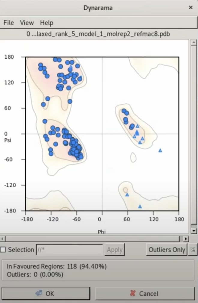
An example of the Ramachandran Plot integrated in COOT used in this tutorial. Compared to the classic Ramachandran plot, the resolution of the Favored/Allowed/Outilers boundary lines has increased.

It should be noted that it is not necessarily required for the model structure to always fall within the Favored region of the Ramachandran Plot. These are merely representations of the statistical average of all proteins, and in cases like the present one, where the electron cloud is clearly visible at high resolution, a structure can be deemed reliable even if it falls in the Outliers, given there is experimental evidence.

For the actual structural modification using COOT, please refer to the video below (played at 5x speed).

The Refmac settings and the log during execution are provided (values at the time the author conducted the process, there should be no issue if the values are around the same).

Step.4-1-9 Cycle.9

Parameter	Value
Refinement method	Restrained Refinement
Resolution	1.3Å
B-factor	Anisotropic
Target	Protein Structure + Water + Ramachandran Plot + Geometory check

Similar to Cycle.8, we made structural modifications with reference to the protein model structure, bound water, and the protein model structure's Ramachandran Plot and Geometry check. Even if the structure is modified and refined with Refmac, be aware that the model structure may change during the Refmac process, and the geometry may revert back to its pre-modification state.

For the actual structural modification using COOT, please refer to the video below (played at 5x speed).

The Refmac settings and the log during execution are provided (values at the time the author conducted the process, there should be no issue if the values are around the same).

Step.4-1-10 Cycle.10

Parameter	Value
Refinement method	Restrained Refinement
Resolution	1.3Å
B-factor	Anisotropic
Target	Protein Structure + Water + Ramachandran Plot + Geometory check

Similar to Cycle.9, minor modifications were made. Also, as the R-factor/R-free values stabilized through repeated modifications, we determined that the desired optimal fitting has been achieved.

For the actual structural modification using COOT, please refer to the video below (played at 5x speed).

The Refmac settings and the log during execution are provided (values at the time the author conducted the process, there should be no issue if the values are around the same).

Step.4-1-11 Cycle.11

Parameter	Value
Refinement method	Restrained Refinement
Resolution	1.3Å
B-factor	Anisotropic
Target	Protein Structure + Water + Ramachandran Plot + Geometory check
Validation	Mol Probity

Ultimately, a comprehensive check of the model structure of Lysozyme was performed using MolProbity, and based on this, the model structure was revised and refined to determine the final protein model structure.

MolProbity is a well-known validation tool for protein model structures. In Phenix.refine, a refinement software of Phenix, which is a structural analysis software suite alongside CCP4, a structural check by the integrated MolProbity is automatically performed after refinement. On the other hand, unfortunately, such a feature is not equipped in Refmac5 of CCP4 used in this tutorial, so a structure check by the Web version of MolProbity will be conducted following the steps below. This is a necessary step when registering a protein model structure to the PDB.

1. Access the Web version of MolProbity, and upload the PDB (or mmCIF) file output in Cycle.10. Then, proceed to the screen at the lower right of the image.
   

2. Click "Analyze geometry without all-atom contacts" to initiate the preprocessing for the analysis, and transition to the selection screen of analysis items at the lower left of the image. For now, the analysis will be conducted with the standard analysis items that are already selected. Click "Run programs to perform these analyses" and carry out the analysis.
   

3. The analysis results are displayed. In Summary statistics, items highlighted in green indicate no issues. On the other hand, items highlighted in red indicate there are issues, so scroll down to understand what the problem is.
   

With these MolProbity results, you will review and correct the structure in COOT.
Please refer to the following video (at 5x speed) for the actual operation.

Here are the setting values for Refmac and the log at execution (values at the time of the author's execution. There are no issues as long as the values are similar).

Step.4-1-12 Determination of Protein Model Structure

It has been a long journey from checking the diffraction image to this point, but by refining the structure based on the validation information from MolProbity and conducting the final refinement with Refmac, we have finally been able to determine the final protein model structure.

When registering the determined structure in the PDB or publishing it in a paper, there is a standard practice to create a table summarizing the statistical values of the structure, colloquially known as "Table.1" in the industry. Although we are not submitting to the PDB or writing a paper in this tutorial, let's go ahead and finish up with creating Table.1. The items listed in Table.1 can vary depending on the creator. Therefore, the numbers shown below are the author's preference, and your understanding is appreciated. If you are unsure about what items to include, it may be helpful to mimic Table.1 in papers published in the specialized journal IUCr Acta Crystallographica Section D.

Below, the author's data is used to create Table.1 for the Lysozyme analyzed in this tutorial. Please use this as a reference.

	Lysozyme	Commentary
Data collection
Diffraction source	NSLS-II 17-ID-2	Step.2: Cited from the information of the diffraction data set used
Wavelength(Å)	0.97894	Step.2: Cited from the information of the diffraction data set used
Resolution range(Å)	39.27-1.30 (1.32-1.30)	Step.2: Cited from the results of Aimless (log)
Space group	P43212	Step.2: Cited from the results of Aimless (log)
a,b,c(Å)	78.54, 78.54, 37.28	Step.2: Cited from the results of Aimless (log)
α, β, γ (°)	90, 90, 90	Step.2: Cited from the results of Aimless (log)
Reflections (measured/unique)	714,243/28,373	Step.2: Cited from the results of Aimless (log)
Completeness (%)	97.1 (89.4)	Step.2: Cited from the results of Aimless (log)
Mean I/σ(I)	65.1 (19.4)	Step.2: Cited from the results of Aimless (log)
Multiplicity	25.2 (19.7)	Step.2: Cited from the results of Aimless (log)
Rpim	0.009 (0.042)	Step.2: Cited from the results of Aimless (log)
CC(1/2)	1.000 (0.996)	Step.2: Cited from the results of Aimless (log)
Wilson B factor (Å2)	10.762	Step.2: Cited from the results of Aimless (log)
Refinement statistics
Resolution range(Å)	35.15-1.30	Step.4: Cited from the final model structure (mmcif,pdb)
R-factor (%)/Rfree(%)	13.16/15.65	Step.4: Cited from the final model structure (mmcif,pdb)
No. of atoms in structure
Protein	1,187	Step.4: Cited from the final model structure (mmcif,pdb)
Ligand	0
Water	159	Step.4: Count HOH columns of cited from the final model structure (mmcif,pdb)
R.m.s deviations from ideal
Bond lengths (Å)	0.011	Step.4: Cited from the final model structure (mmcif,pdb)
Bond angles(°)	1.78	Step.4: Cited from the final model structure (mmcif,pdb)
Chiral volumes(Å$^3$)	0.114	Step.4: Cited from the final model structure (mmcif,pdb)
Ramachandran plot, residues in (%)
Most favorable region	98.5	Step.4: Cited from MolProbity result of final refinement protein model
Additional allowed region	100.0	Step.4: Cited from MolProbity result of final refinement protein model
Average B factor(Å$^2$)	13.559	Step.4: Cited from the final model structure (mmcif,pdb)

(Values in parentheses are for the outer shell.)

With the creation of Table.1, the structure refinement is now complete. Excellent work and well done.

The author has uploaded the results of the structure refinement performed using Refmac5 on GitHub. You are highly encouraged to refer to it.

Visualization with Pymol

As an additional note, since we have performed structure analysis, let's create a high-quality diagram of the protein model structure using Pymol, a standard protein model visualization software, that can be used for presentations.

This article will not delve into details about Pymol. The Protein Research Institute of Osaka University's Guide on How to Use PyMOL (GUI ver.)(JP) provides a comprehensive guide, so I strongly recommend referring to it.

For the actual operation, please refer to the following video (5x speed).

Conclusion

This concludes the Lysozyme X-ray crystal structure analysis tutorial composed of Step.1 ~ Step.4. For experienced users, the process may have seemed routine. However, for beginners, it might have been challenging due to the myriad of things to learn, including prerequisite knowledge. The author, too, was surprised by how intricate and advanced the process was when trying to put it into words. Great job making it through!

As of March 2023, when this article was written, it is believed that full automation of protein X-ray crystal structure analysis is difficult due to the need for advanced judgment at various stages. However, with the recent rapid advancement in AI, as exemplified by image generation models (like Stable Diffusion) and large language models (like GPT3, Chat-GPT), it's believed that a future where a refined structure can be output just by feeding in diffraction image datasets and the amino acid sequence (in fasta format, for instance) of the target protein is not far off. It's also considered desirable. This belief led to the writing of this article, intending to have those with machine learning expertise first understand the reality of traditional manual protein X-ray crystal structure analysis.

Looking back at the first edition, it seems like this article could be an ideal introductory guide for students and researchers tackling protein X-ray crystal structure analysis for the first time. It would be a pleasure if it could be of help to many people.

While this tutorial has been written with the utmost attention to accuracy, it may contain errors or oversights when viewed by a domain expert. Comments or suggestions to improve this article, such as through the Qiita comment section, would be highly appreciated.

In Step.4, CCP4's Refmac was used, but in reality, the author is more proficient in structure refinement using Phenix. There are plans to write an additional article about structure refinement using Phenix as an extra section to Step.4 (presumably).

Lastly, this article owes much to the capabilities of ChatGPT/BingGPT provided by OpenAI/Microsoft. I would like to express my gratitude to the researchers and developers whose blood and sweat have contributed to these developments.

Reference

• 2022 DLS-CCP4 Data Collection and Structure Solution Workshop Course Material - Refinement with Refmac
• PDB-101: R-value and R-free
• The phase problem. Garry Taylor, Acta Crystallographica Section D, Volume 59| Part 11| November 2003| Pages 1881-1890

Table of Contents

• Step.0 The flow of structure determination
• Step.1 Installing analytical software
• Step.2 Checking diffraction images and calculating structure factors
• Step.3 Finding initial phases
• Step.4 Structure refinement and validation (This article)

1. Indeed, even when looking at the electron density cloud ρ(xyz) at a resolution of 1.3Å, it would seem difficult to unambiguously determine the position of each atom. ↩