(目次はこちら)
(Tensorflow 2.0版: https://qiita.com/kumonkumon/items/337796dae8d42ce36fa8)

はじめに

前回の記事では、多項ロジスティック回帰について扱った。これは、 TensorFlowのTutorialのMNIST For ML Beginners ほぼそのままなので全く面白くないので少し拡張してみる。(追記: MNIST For ML Beginnersは2019年時点ではもうありません)

MNIST For ML Beginners では、

This should be about 91%.

Is that good? Well, not really. In fact, it's pretty bad. This is because we're using a very simple model. With some small changes, we can get to 97%

「多項ロジスティック回帰では、91%くらいの精度で、いい結果じゃないよ、少し変えれば97%くらいいくよ。」と。

ただ、この、

With some small changes

がなんなのかは書いていないので、ちょっと何か試してみる。

多層パーセプトロン（multilayer perceptron）

多項ロジスティック回帰を、多層パーセプトロンへと拡張してみる。

画像に限らず、何かのデータを識別するときには、「入力データから特徴抽出して識別器にかける」というのが王道。
前回の記事では、入力データを直接識別器にかけて認識していたので、入力データそのもの、すなわち、画像の画素値そのものが特徴として扱われていたことになる。

今回は、特徴抽出部分を追加してみる。特徴抽出といってもやり方はいろいろあって、

エッジ抽出フィルタ
SIFT
SURF
etc...

などなど、、でも、ここでは、画像にとらわれない特徴抽出的な層を一つ追加することにする。「特徴抽出的な層」っと言ってもなんのことやらだけど、多項ロジスティック回帰の中に、「特徴抽出的な層」としてロジスティック回帰をねじ込んでみる。

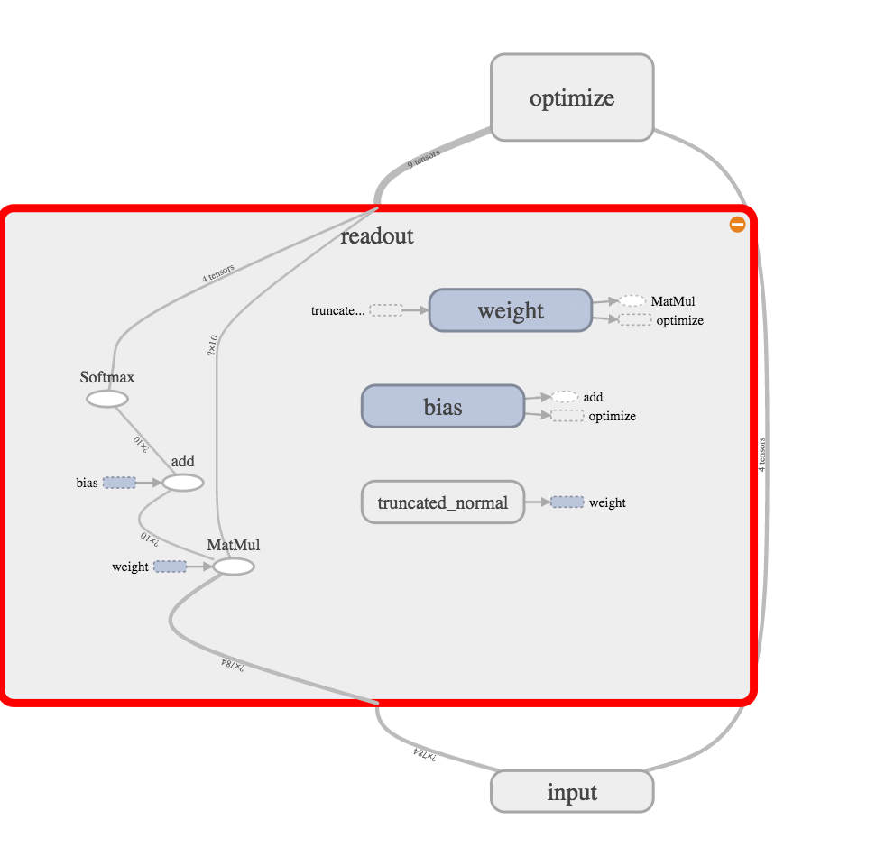
前回の記事での、多項ロジスティック回帰はこんな感じ。

で、多項ロジスティック回帰にロジスティック回帰をねじ込む。

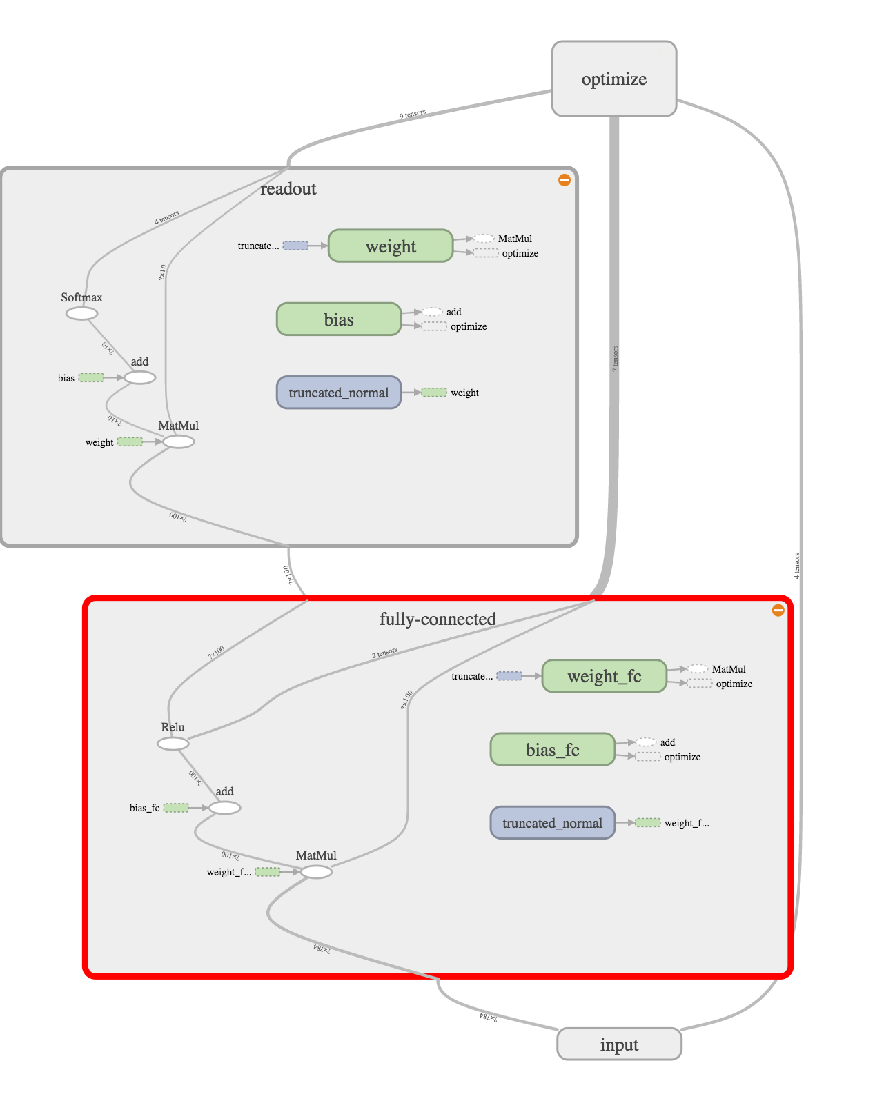
readout layerとinput layerの間に、fully-conneced layer（全結合層）というのがねじ込まれている。で、よく見てみると、入力を線形変換してReLU（ランプ関数）という活性化関数にかけて、その結果をreadout layerに入れていることがわかる。

これは、活性化関数にステップ関数を使っていないのでパーセプトロンではないけど、多層パーセプトロン（multilayer perceptron）とよばれているもの。ここまでくるとニューラルネットワークっぽくなった。

コード

Python: 3.6.8, Tensorflow: 1.13.1で動作確認済み
(もともと2016年前半に書いたものなので、順次更新しています。)

mnist_softmax_fc.py

from helper import *

IMAGE_SIZE = 28 * 28
CATEGORY_NUM = 10
LEARNING_RATE = 0.1
FEATURE_DIM = 100
TRAINING_LOOP = 20000
BATCH_SIZE = 100
SUMMARY_DIR = 'log_softmax_fc'
SUMMARY_INTERVAL = 1000
BUFFER_SIZE = 1000
EPS = 1e-10


with tf.Graph().as_default():
    (X_train, y_train), (X_test, y_test) = mnist_samples(flatten_image=True)
    ds = tf.data.Dataset.from_tensor_slices((X_train, y_train))
    ds = ds.shuffle(BUFFER_SIZE).batch(BATCH_SIZE).repeat(int(TRAINING_LOOP * BATCH_SIZE / X_train.shape[0]) + 1)
    next_batch = ds.make_one_shot_iterator().get_next()

    with tf.name_scope('input'):
        y_ = tf.placeholder(tf.float32, [None, CATEGORY_NUM], name='labels')
        x = tf.placeholder(tf.float32, [None, IMAGE_SIZE], name='input_images')

    with tf.name_scope('fully-connected'):
        W_fc = weight_variable([IMAGE_SIZE, FEATURE_DIM], name='weight_fc')
        b_fc = bias_variable([FEATURE_DIM], name='bias_fc')
        h_fc = tf.nn.relu(tf.matmul(x, W_fc) + b_fc)

    with tf.name_scope('readout'):
        W = weight_variable([FEATURE_DIM, CATEGORY_NUM], name='weight')
        b = bias_variable([CATEGORY_NUM], name='bias')
        y = tf.nn.softmax(tf.matmul(h_fc, W) + b)

    with tf.name_scope('optimize'):
        y = tf.clip_by_value(y, EPS, 1.0)
        cross_entropy = -tf.reduce_mean(tf.reduce_sum(y_ * tf.log(y), axis=1))
        train_step = tf.train.GradientDescentOptimizer(LEARNING_RATE).minimize(cross_entropy)
        cross_entropy_summary = tf.summary.scalar('cross entropy', cross_entropy)

    with tf.Session() as sess:
        train_writer = tf.summary.FileWriter(SUMMARY_DIR + '/train', sess.graph)
        test_writer = tf.summary.FileWriter(SUMMARY_DIR + '/test')

        correct_prediction = tf.equal(tf.argmax(y, 1), tf.argmax(y_, 1))
        accuracy = tf.reduce_mean(tf.cast(correct_prediction, tf.float32))
        accuracy_summary = tf.summary.scalar('accuracy', accuracy)

        sess.run(tf.global_variables_initializer())
        for i in range(TRAINING_LOOP + 1):
            images, labels = sess.run(next_batch)
            sess.run(train_step, {x: images, y_: labels})

            if i % SUMMARY_INTERVAL == 0:
                train_acc, summary = sess.run(
                        [accuracy, tf.summary.merge([cross_entropy_summary, accuracy_summary])],
                        {x: images, y_: labels})
                train_writer.add_summary(summary, i)
                test_acc, summary = sess.run(
                        [accuracy, tf.summary.merge([cross_entropy_summary, accuracy_summary])],
                        {x: X_test, y_: y_test})
                test_writer.add_summary(summary, i)
                print(f'step: {i}, train-acc: {train_acc}, test-acc: {test_acc}')

コードの説明

多項ロジスティック回帰と異なる部分を。

全結合層

追加された層。入力データを線形変換してReLUという活性化関数を通っている。FEATURE_DIMは出力を何次元にするか（何次元の特徴ベクトルにするか）のパラメータ。

with tf.name_scope('fully-connected'):
    W_fc = weight_variable([IMAGE_SIZE, FEATURE_DIM], name='weight_fc')
    b_fc = bias_variable([FEATURE_DIM], name='bias_fc')
    h_fc = tf.nn.relu(tf.matmul(x, W_fc) + b_fc)

出力層

入力が全結合層の出力となるように変更。

with tf.name_scope('readout'):
    W = weight_variable([FEATURE_DIM, CATEGORY_NUM], name='weight')
    b = bias_variable([CATEGORY_NUM], name='bias')
    y = tf.nn.softmax(tf.matmul(h_fc, W) + b)

以上です。変更量は非常に少ない。

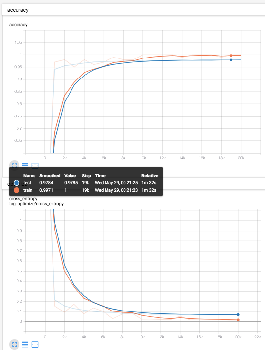
結果

テストデータ（青線）での識別率は、97.8%程度。
前回の記事での、多項ロジスティック回帰での結果が、92.4%程度だったのでかなり改善している。

あとがき

今回は、多項ロジスティック回帰を拡張して、多層パーセプトロンにしてみました。次回の記事では、畳み込みニューラルネットワーク（Convolutional Neural Network：CNN）に足を踏み入れてみます。

多層パーセプトロン [TensorFlowでDeep Learning 3]

はじめに

多層パーセプトロン（multilayer perceptron）

コード

コードの説明

全結合層

出力層

結果

あとがき