「ラビットチャレンジ」 提出レポート
1.機械学習とは
■ (トム・ミッチェル 1997)の定義
コンピュータプログラムはタスク $T$ とパフォーマンス測定 $P$ に関連する経験 $E$ から学習すると言われています。タスク $T$ でパフォーマンスをした場合、パフォーマンス測定 $P$ によって達成度が測定され、経験 $E$ によって改善されていきます。
■ 機械学習モデリングプロセス
● Step 1 :問題設定(どのような課題を機械学習に解決させるか)
● Step 2 :データ選定(どのようなデータを使うか)
● Step 3 :データの前処理(モデルに学習させられるようにデータを加工する)
● Step 4 :機械学習モデルの選定(どの機械学習モデルを利用するか)
● Step 5 :モデルの学習(パラメータ推定)
● Step 6 :モデル評価(ハイパーパラメータの選定、モデル精度を測る)
2.線形回帰モデル
■ **回帰問題:**離散値あるいは連続値の入力から連続値の出力を予測する
■ **回帰で扱うデータ:**説明変数または特徴量(入力)と目的変数(出力)
■ **線形回帰モデル:**教師あり学習で、入力と $m$ 次元パラメータの線形結合を出力するモデル($m=1$の場合、単回帰モデルという)
■ **線形結合:**入力とパラメータの内積
● パラメータ: $w$ = ($w_1$ ,$w_2$ ,・・・,$w_m$)$^T$ $\subset$ $\mathbb{R}^m$
● 説明変数:$\quad$$x$ = ($x_1$ ,$x_2$ ,・・・,$x_m$)$^T$ $\subset$ $\mathbb{R}^m$
● 線形結合:
\hat{y} = w^Tx + w_0= \sum_{j=1}^{m} w_jx_j + w_0
そこで、$\hat{y}$ は予測値という。
3.データ分割・学習
■ データ分割: モデルの汎化性能を測定するため、データを学習用データと検証用データに分割する
■ 最小二乗法:
● 学習データの平均二乗誤差を最小とするパラメータを探索する
● 学習データの平均二乗誤差を最小は、その勾配が0になる点を求めれば良い。
● 学習データの平均二乗誤差は次式の通りに書きます。
MSE_{train} = \frac{1}{n_{train}}\sum_{i=1}^{n_{train}}(\hat{y}_i^{(train)}-y_i^{(train)})^2
4.ハンズオン
【演習実施結果】線形回帰モデル-Boston Hausing Data-
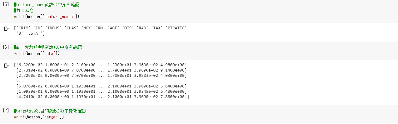
■ 必要モジュールとデータのインポート

{'data': array([[6.3200e-03, 1.8000e+01, 2.3100e+00, ..., 1.5300e+01, 3.9690e+02,
        4.9800e+00],
       [2.7310e-02, 0.0000e+00, 7.0700e+00, ..., 1.7800e+01, 3.9690e+02,
        9.1400e+00],
       [2.7290e-02, 0.0000e+00, 7.0700e+00, ..., 1.7800e+01, 3.9283e+02,
        4.0300e+00],
       ...,
       [6.0760e-02, 0.0000e+00, 1.1930e+01, ..., 2.1000e+01, 3.9690e+02,
        5.6400e+00],
       [1.0959e-01, 0.0000e+00, 1.1930e+01, ..., 2.1000e+01, 3.9345e+02,
        6.4800e+00],
       [4.7410e-02, 0.0000e+00, 1.1930e+01, ..., 2.1000e+01, 3.9690e+02,
        7.8800e+00]]), 'target': array([24. , 21.6, 34.7, 33.4, 36.2, 28.7, 22.9, 27.1, 16.5, 18.9, 15. ,
       18.9, 21.7, 20.4, 18.2, 19.9, 23.1, 17.5, 20.2, 18.2, 13.6, 19.6,
       15.2, 14.5, 15.6, 13.9, 16.6, 14.8, 18.4, 21. , 12.7, 14.5, 13.2,
       13.1, 13.5, 18.9, 20. , 21. , 24.7, 30.8, 34.9, 26.6, 25.3, 24.7,
       21.2, 19.3, 20. , 16.6, 14.4, 19.4, 19.7, 20.5, 25. , 23.4, 18.9,
       35.4, 24.7, 31.6, 23.3, 19.6, 18.7, 16. , 22.2, 25. , 33. , 23.5,
       19.4, 22. , 17.4, 20.9, 24.2, 21.7, 22.8, 23.4, 24.1, 21.4, 20. ,
       20.8, 21.2, 20.3, 28. , 23.9, 24.8, 22.9, 23.9, 26.6, 22.5, 22.2,
       23.6, 28.7, 22.6, 22. , 22.9, 25. , 20.6, 28.4, 21.4, 38.7, 43.8,
       33.2, 27.5, 26.5, 18.6, 19.3, 20.1, 19.5, 19.5, 20.4, 19.8, 19.4,
       21.7, 22.8, 18.8, 18.7, 18.5, 18.3, 21.2, 19.2, 20.4, 19.3, 22. ,
       20.3, 20.5, 17.3, 18.8, 21.4, 15.7, 16.2, 18. , 14.3, 19.2, 19.6,
       23. , 18.4, 15.6, 18.1, 17.4, 17.1, 13.3, 17.8, 14. , 14.4, 13.4,
       15.6, 11.8, 13.8, 15.6, 14.6, 17.8, 15.4, 21.5, 19.6, 15.3, 19.4,
       17. , 15.6, 13.1, 41.3, 24.3, 23.3, 27. , 50. , 50. , 50. , 22.7,
       25. , 50. , 23.8, 23.8, 22.3, 17.4, 19.1, 23.1, 23.6, 22.6, 29.4,
       23.2, 24.6, 29.9, 37.2, 39.8, 36.2, 37.9, 32.5, 26.4, 29.6, 50. ,
       32. , 29.8, 34.9, 37. , 30.5, 36.4, 31.1, 29.1, 50. , 33.3, 30.3,
       34.6, 34.9, 32.9, 24.1, 42.3, 48.5, 50. , 22.6, 24.4, 22.5, 24.4,
       20. , 21.7, 19.3, 22.4, 28.1, 23.7, 25. , 23.3, 28.7, 21.5, 23. ,
       26.7, 21.7, 27.5, 30.1, 44.8, 50. , 37.6, 31.6, 46.7, 31.5, 24.3,
       31.7, 41.7, 48.3, 29. , 24. , 25.1, 31.5, 23.7, 23.3, 22. , 20.1,
       22.2, 23.7, 17.6, 18.5, 24.3, 20.5, 24.5, 26.2, 24.4, 24.8, 29.6,
       42.8, 21.9, 20.9, 44. , 50. , 36. , 30.1, 33.8, 43.1, 48.8, 31. ,
       36.5, 22.8, 30.7, 50. , 43.5, 20.7, 21.1, 25.2, 24.4, 35.2, 32.4,
       32. , 33.2, 33.1, 29.1, 35.1, 45.4, 35.4, 46. , 50. , 32.2, 22. ,
       20.1, 23.2, 22.3, 24.8, 28.5, 37.3, 27.9, 23.9, 21.7, 28.6, 27.1,
       20.3, 22.5, 29. , 24.8, 22. , 26.4, 33.1, 36.1, 28.4, 33.4, 28.2,
       22.8, 20.3, 16.1, 22.1, 19.4, 21.6, 23.8, 16.2, 17.8, 19.8, 23.1,
       21. , 23.8, 23.1, 20.4, 18.5, 25. , 24.6, 23. , 22.2, 19.3, 22.6,
       19.8, 17.1, 19.4, 22.2, 20.7, 21.1, 19.5, 18.5, 20.6, 19. , 18.7,
       32.7, 16.5, 23.9, 31.2, 17.5, 17.2, 23.1, 24.5, 26.6, 22.9, 24.1,
       18.6, 30.1, 18.2, 20.6, 17.8, 21.7, 22.7, 22.6, 25. , 19.9, 20.8,
       16.8, 21.9, 27.5, 21.9, 23.1, 50. , 50. , 50. , 50. , 50. , 13.8,
       13.8, 15. , 13.9, 13.3, 13.1, 10.2, 10.4, 10.9, 11.3, 12.3,  8.8,
        7.2, 10.5,  7.4, 10.2, 11.5, 15.1, 23.2,  9.7, 13.8, 12.7, 13.1,
       12.5,  8.5,  5. ,  6.3,  5.6,  7.2, 12.1,  8.3,  8.5,  5. , 11.9,
       27.9, 17.2, 27.5, 15. , 17.2, 17.9, 16.3,  7. ,  7.2,  7.5, 10.4,
        8.8,  8.4, 16.7, 14.2, 20.8, 13.4, 11.7,  8.3, 10.2, 10.9, 11. ,
        9.5, 14.5, 14.1, 16.1, 14.3, 11.7, 13.4,  9.6,  8.7,  8.4, 12.8,
       10.5, 17.1, 18.4, 15.4, 10.8, 11.8, 14.9, 12.6, 14.1, 13. , 13.4,
       15.2, 16.1, 17.8, 14.9, 14.1, 12.7, 13.5, 14.9, 20. , 16.4, 17.7,
       19.5, 20.2, 21.4, 19.9, 19. , 19.1, 19.1, 20.1, 19.9, 19.6, 23.2,
       29.8, 13.8, 13.3, 16.7, 12. , 14.6, 21.4, 23. , 23.7, 25. , 21.8,
       20.6, 21.2, 19.1, 20.6, 15.2,  7. ,  8.1, 13.6, 20.1, 21.8, 24.5,
       23.1, 19.7, 18.3, 21.2, 17.5, 16.8, 22.4, 20.6, 23.9, 22. , 11.9]), 'feature_names': array(['CRIM', 'ZN', 'INDUS', 'CHAS', 'NOX', 'RM', 'AGE', 'DIS', 'RAD',
       'TAX', 'PTRATIO', 'B', 'LSTAT'], dtype='<U7'), 'DESCR': ".. _boston_dataset:\n\nBoston house prices dataset\n---------------------------\n\n**Data Set Characteristics:**  \n\n    :Number of Instances: 506 \n\n    :Number of Attributes: 13 numeric/categorical predictive. Median Value (attribute 14) is usually the target.\n\n    :Attribute Information (in order):\n        - CRIM     per capita crime rate by town\n        - ZN       proportion of residential land zoned for lots over 25,000 sq.ft.\n        - INDUS    proportion of non-retail business acres per town\n        - CHAS     Charles River dummy variable (= 1 if tract bounds river; 0 otherwise)\n        - NOX      nitric oxides concentration (parts per 10 million)\n        - RM       average number of rooms per dwelling\n        - AGE      proportion of owner-occupied units built prior to 1940\n        - DIS      weighted distances to five Boston employment centres\n        - RAD      index of accessibility to radial highways\n        - TAX      full-value property-tax rate per $10,000\n        - PTRATIO  pupil-teacher ratio by town\n        - B        1000(Bk - 0.63)^2 where Bk is the proportion of blacks by town\n        - LSTAT    % lower status of the population\n        - MEDV     Median value of owner-occupied homes in $1000's\n\n    :Missing Attribute Values: None\n\n    :Creator: Harrison, D. and Rubinfeld, D.L.\n\nThis is a copy of UCI ML housing dataset.\nhttps://archive.ics.uci.edu/ml/machine-learning-databases/housing/\n\n\nThis dataset was taken from the StatLib library which is maintained at Carnegie Mellon University.\n\nThe Boston house-price data of Harrison, D. and Rubinfeld, D.L. 'Hedonic\nprices and the demand for clean air', J. Environ. Economics & Management,\nvol.5, 81-102, 1978.   Used in Belsley, Kuh & Welsch, 'Regression diagnostics\n...', Wiley, 1980.   N.B. Various transformations are used in the table on\npages 244-261 of the latter.\n\nThe Boston house-price data has been used in many machine learning papers that address regression\nproblems.   \n     \n.. topic:: References\n\n   - Belsley, Kuh & Welsch, 'Regression diagnostics: Identifying Influential Data and Sources of Collinearity', Wiley, 1980. 244-261.\n   - Quinlan,R. (1993). Combining Instance-Based and Model-Based Learning. In Proceedings on the Tenth International Conference of Machine Learning, 236-243, University of Massachusetts, Amherst. Morgan Kaufmann.\n", 'filename': '/usr/local/lib/python3.6/dist-packages/sklearn/datasets/data/boston_house_prices.csv'}

.. _boston_dataset:

Boston house prices dataset
---------------------------

**Data Set Characteristics:**

    :Number of Instances: 506

    :Number of Attributes: 13 numeric/categorical predictive. Median Value (attribute 14) is usually the target.

    :Attribute Information (in order):
        - CRIM     per capita crime rate by town
        - ZN       proportion of residential land zoned for lots over 25,000 sq.ft.
        - INDUS    proportion of non-retail business acres per town
        - CHAS     Charles River dummy variable (= 1 if tract bounds river; 0 otherwise)
        - NOX      nitric oxides concentration (parts per 10 million)
        - RM       average number of rooms per dwelling
        - AGE      proportion of owner-occupied units built prior to 1940
        - DIS      weighted distances to five Boston employment centres
        - RAD      index of accessibility to radial highways
        - TAX      full-value property-tax rate per $10,000
        - PTRATIO  pupil-teacher ratio by town
        - B        1000(Bk - 0.63)^2 where Bk is the proportion of blacks by town
        - LSTAT    % lower status of the population
        - MEDV     Median value of owner-occupied homes in $1000's

    :Missing Attribute Values: None

    :Creator: Harrison, D. and Rubinfeld, D.L.

This is a copy of UCI ML housing dataset.
https://archive.ics.uci.edu/ml/machine-learning-databases/housing/


This dataset was taken from the StatLib library which is maintained at Carnegie Mellon University.

The Boston house-price data of Harrison, D. and Rubinfeld, D.L. 'Hedonic
prices and the demand for clean air', J. Environ. Economics & Management,
vol.5, 81-102, 1978.   Used in Belsley, Kuh & Welsch, 'Regression diagnostics
...', Wiley, 1980.   N.B. Various transformations are used in the table on
pages 244-261 of the latter.

The Boston house-price data has been used in many machine learning papers that address regression
problems.

.. topic:: References

   - Belsley, Kuh & Welsch, 'Regression diagnostics: Identifying Influential Data and Sources of Collinearity', Wiley, 1980. 244-261.
   - Quinlan,R. (1993). Combining Instance-Based and Model-Based Learning. In Proceedings on the Tenth International Conference of Machine Learning, 236-243, University of Massachusetts, Amherst. Morgan Kaufmann.
[24.  21.6 34.7 33.4 36.2 28.7 22.9 27.1 16.5 18.9 15.  18.9 21.7 20.4
 18.2 19.9 23.1 17.5 20.2 18.2 13.6 19.6 15.2 14.5 15.6 13.9 16.6 14.8
 18.4 21.  12.7 14.5 13.2 13.1 13.5 18.9 20.  21.  24.7 30.8 34.9 26.6
 25.3 24.7 21.2 19.3 20.  16.6 14.4 19.4 19.7 20.5 25.  23.4 18.9 35.4
 24.7 31.6 23.3 19.6 18.7 16.  22.2 25.  33.  23.5 19.4 22.  17.4 20.9
 24.2 21.7 22.8 23.4 24.1 21.4 20.  20.8 21.2 20.3 28.  23.9 24.8 22.9
 23.9 26.6 22.5 22.2 23.6 28.7 22.6 22.  22.9 25.  20.6 28.4 21.4 38.7
 43.8 33.2 27.5 26.5 18.6 19.3 20.1 19.5 19.5 20.4 19.8 19.4 21.7 22.8
 18.8 18.7 18.5 18.3 21.2 19.2 20.4 19.3 22.  20.3 20.5 17.3 18.8 21.4
 15.7 16.2 18.  14.3 19.2 19.6 23.  18.4 15.6 18.1 17.4 17.1 13.3 17.8
 14.  14.4 13.4 15.6 11.8 13.8 15.6 14.6 17.8 15.4 21.5 19.6 15.3 19.4
 17.  15.6 13.1 41.3 24.3 23.3 27.  50.  50.  50.  22.7 25.  50.  23.8
 23.8 22.3 17.4 19.1 23.1 23.6 22.6 29.4 23.2 24.6 29.9 37.2 39.8 36.2
 37.9 32.5 26.4 29.6 50.  32.  29.8 34.9 37.  30.5 36.4 31.1 29.1 50.
 33.3 30.3 34.6 34.9 32.9 24.1 42.3 48.5 50.  22.6 24.4 22.5 24.4 20.
 21.7 19.3 22.4 28.1 23.7 25.  23.3 28.7 21.5 23.  26.7 21.7 27.5 30.1
 44.8 50.  37.6 31.6 46.7 31.5 24.3 31.7 41.7 48.3 29.  24.  25.1 31.5
 23.7 23.3 22.  20.1 22.2 23.7 17.6 18.5 24.3 20.5 24.5 26.2 24.4 24.8
 29.6 42.8 21.9 20.9 44.  50.  36.  30.1 33.8 43.1 48.8 31.  36.5 22.8
 30.7 50.  43.5 20.7 21.1 25.2 24.4 35.2 32.4 32.  33.2 33.1 29.1 35.1
 45.4 35.4 46.  50.  32.2 22.  20.1 23.2 22.3 24.8 28.5 37.3 27.9 23.9
 21.7 28.6 27.1 20.3 22.5 29.  24.8 22.  26.4 33.1 36.1 28.4 33.4 28.2
 22.8 20.3 16.1 22.1 19.4 21.6 23.8 16.2 17.8 19.8 23.1 21.  23.8 23.1
 20.4 18.5 25.  24.6 23.  22.2 19.3 22.6 19.8 17.1 19.4 22.2 20.7 21.1
 19.5 18.5 20.6 19.  18.7 32.7 16.5 23.9 31.2 17.5 17.2 23.1 24.5 26.6
 22.9 24.1 18.6 30.1 18.2 20.6 17.8 21.7 22.7 22.6 25.  19.9 20.8 16.8
 21.9 27.5 21.9 23.1 50.  50.  50.  50.  50.  13.8 13.8 15.  13.9 13.3
 13.1 10.2 10.4 10.9 11.3 12.3  8.8  7.2 10.5  7.4 10.2 11.5 15.1 23.2
  9.7 13.8 12.7 13.1 12.5  8.5  5.   6.3  5.6  7.2 12.1  8.3  8.5  5.
 11.9 27.9 17.2 27.5 15.  17.2 17.9 16.3  7.   7.2  7.5 10.4  8.8  8.4
 16.7 14.2 20.8 13.4 11.7  8.3 10.2 10.9 11.   9.5 14.5 14.1 16.1 14.3
 11.7 13.4  9.6  8.7  8.4 12.8 10.5 17.1 18.4 15.4 10.8 11.8 14.9 12.6
 14.1 13.  13.4 15.2 16.1 17.8 14.9 14.1 12.7 13.5 14.9 20.  16.4 17.7
 19.5 20.2 21.4 19.9 19.  19.1 19.1 20.1 19.9 19.6 23.2 29.8 13.8 13.3
 16.7 12.  14.6 21.4 23.  23.7 25.  21.8 20.6 21.2 19.1 20.6 15.2  7.
  8.1 13.6 20.1 21.8 24.5 23.1 19.7 18.3 21.2 17.5 16.8 22.4 20.6 23.9
 22.  11.9]
■ データフレームの作成

■ 線形単回帰分析


**【結果】**上記の予測結果を見ると、一戸あたりの平均部屋数が1の場合、住宅価格は[-25.5685118]となる.また、一戸あたりの平均部屋数が4の場合、住宅価格は以下になります。

■ 重回帰分析(2変数)
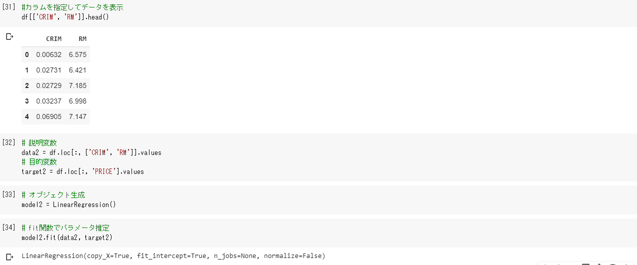


**【結果】**上記の予測結果を見ると、一戸あたりの平均部屋数が7、犯罪発生率 0.2 の場合、住宅価格は[29.43977562]。また、一戸あたりの平均部屋数が4、犯罪発生率 0.3 の場合、住宅価格[4.24007956]
■ 回帰係数と切片の値を確認
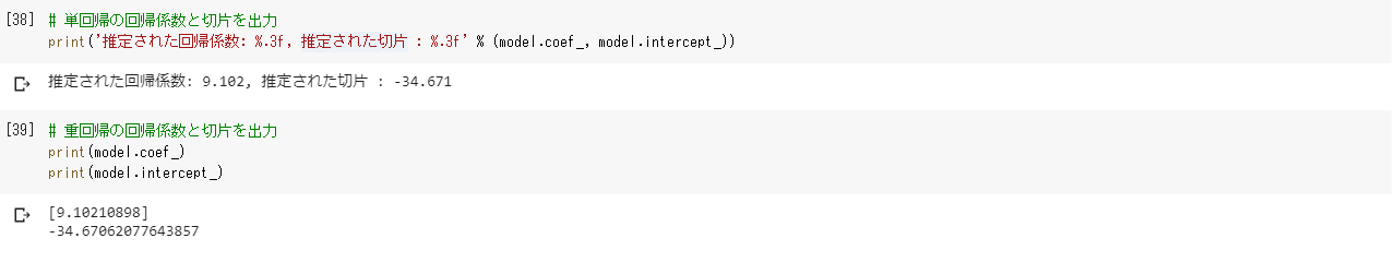
■ モデルの検証


【考察】
■ 下記の結果より、重回帰の方が精度が良いと言える。
(単回帰決定係数: 0.483, 重回帰決定係数 : 0.542)

5.演習問題関連
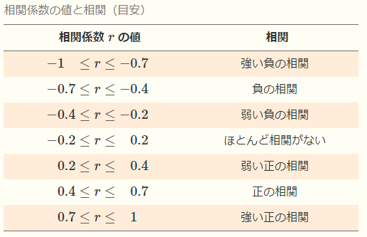
相関係数について
相関係数とは、2 種類のデータの関係を示す指標です。相関係数は無単位なので、単位の影響を受けずにデータの関連性を示します。相関係数は -1 から 1 までの値を取ります。
リッジ回帰、ラッソ回帰について
重回帰分析の損失関数に正則化項を加えたものがリッジ回帰、及びラッソ回帰になります。リッジ回帰では$L2$ノルムの二乗、ラッソ回帰では$L1$ノルムを正則化項として使います。
【機械学習】レポート一覧
【ラビットチャレンジ】【機械学習】非線形回帰モデル
【ラビットチャレンジ】【機械学習】ロジスティク回帰モデル
【ラビットチャレンジ】【機械学習】主成分分析
【ラビットチャレンジ】【機械学習】アルゴリズム
【ラビットチャレンジ】【機械学習】サポートベクターマシン