はじめに
『機械学習のエッセンス(http://isbn.sbcr.jp/93965/)』のPythonサンプルをJuliaで書き換えてみる。(第05章03リッジ回帰)の続きです。
多項式回帰
本の説明の要約です。
y = w_0 + w_1x + w_2x^2 + \cdots + w_dx^d + \varepsilon
$\varepsilon$はノイズ。
\hat{y} = w_0 + w_1x + \cdots + w_dx^d
を$x$と$w$の関数$\hat{y}(x,w)$と見なして、訓練データの特徴量$x$とターゲット$y$に対して次を計算する。
\min_w||\hat{y}(x, w) - y||^2
これは、与えられた訓練データの特徴量$(x_1,x_2,\cdots,x_n)^T$について各要素の$1$から$d$のベキまでを並べた行列
M = \left(
\begin{array}{cccc}
  1 & x_1 & x_{1}^2 & \ldots & x_{1}^d \\
  1 & x_2 & x_{2}^2 & \ldots & x_{2}^d \\
  \vdots & \vdots & \ddots & \vdots \\
  1 & x_n & x_{n}^2 & \ldots & x_{n}^d
\end{array}
\right)
を訓練データの特徴量行列として線形回帰を計算した場合と同じ。
$\hat{y} = (y_1, y_2, \cdots, y_n)$とすると、次のようになる。
\hat{y} = \left(
\begin{array}{cccc}
  w_0 + w_{1}x_{1} + w_{2}x_{1}^2 \ldots + w_{d}x_{1}^d \\
  w_0 + w_{1}x_{2} + w_{2}x_{2}^2 \ldots + w_{d}x_{2}^d  \\
  \vdots  \\
  w_0 + w_{1}x_{n} + w_{2}x_{n}^2 \ldots + w_{d}x_{n}^d
\end{array}
\right)
 = \left(
\begin{array}{cccc}
  1 & x_1 & x_{1}^2 & \ldots & x_{1}^d \\
  1 & x_2 & x_{2}^2 & \ldots & x_{2}^d \\
  \vdots & \vdots & \ddots & \vdots \\
  1 & x_n & x_{n}^2 & \ldots & x_{n}^d
\end{array}
\right)
\left(
\begin{array}{cccc}
  w_0  \\
  w_1  \\
  \vdots  \\
  w_d
\end{array}
\right)
=
Mw
多項式回帰の実装
include("linearreg.jl")

module polyreg
using ..linearreg

mutable struct PolynomialRegression
  degree::Int
  w_
  function PolynomialRegression(degree::Int)
    new(degree, Nothing)
  end
end

function fit(s::PolynomialRegression, x, y)
  x_pow = []
  xx = vec(x)
  for i in 1:s.degree
    push!(x_pow, xx.^i)
  end
  mat = hcat(x_pow...)
  linreg = linearreg.LinearRegression()
  linearreg.fit(linreg, mat, y)
  s.w_ = linreg.w_
end

function predict(s::PolynomialRegression, x)
  r = 0
  for i in 0:s.degree
    r = r .+ x.^i .* s.w_[i+1]
  end
  return r
end

end
-
moduleから同じディレクトリのlinearreg.jlファイルのlinearregモジュールを読み込むときは..linearregとする必要がありました。 - 今まで他の
.jlファイルを読み込むときはREPLでinclude("linearreg.jl")と実行していましたが、ファイルの先頭に書くことができるので今回はそうしました。
include("polyreg.jl")
using .polyreg
using .linearreg
using Random
using Plots

Random.seed!(0)

f(x) = 1 .+ 2 .* x

x = rand(10) * 10
y = f(x) .+ randn(10)

# 多項式回帰
model = polyreg.PolynomialRegression(10)
polyreg.fit(model, x, y)

plt_p_1 = scatter(x, y, color="black", ylim=(minimum(y) - 1, maximum(y) + 1), label="")
xx = LinRange(minimum(x), maximum(x), 300)
yy = [polyreg.predict(model, u) for u in xx]

plt_p_2 = plot!(plt_p_1, xx, yy, color="black", label="")

# 線形回帰
model = linearreg.LinearRegression()
linearreg.fit(model, x, y)
x1 = minimum(x) - 1
x2 = maximum(x) + 1

plot!(plt_p_2, [x1, x2], [f(x1), f(x2)], color="black", linestyle=:dash, label="")
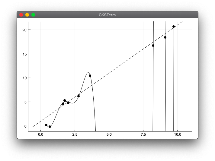
実行結果
julia> include("polyreg_test1.jl")
本では実行時に警告が出ると書いてありますが、Juliaで実行したところ特に警告は出てきませんでした。
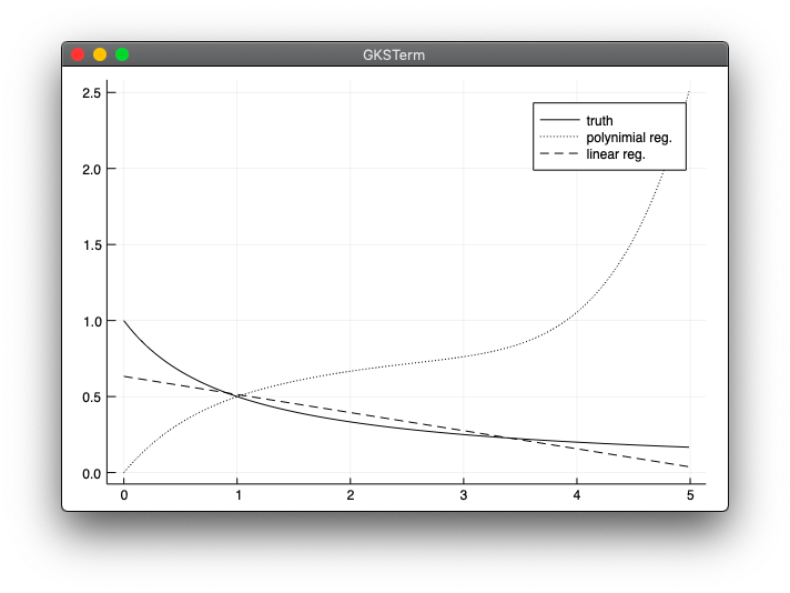
モデルの汎化性能
y = \frac{1}{1 + x} \ \ (0 \le x \le 5)
線形回帰と多項式回帰を使った予測
include("polyreg.jl")
using .linearreg
using .polyreg
using Random
using Plots

f(x) = 1 ./ (1 .+ x)

function sample(n)
    x = rand(n) * 5
    y = f(x)
    return x, y
end

xx = collect(0:0.01:4.99)
Random.seed!(0)
y_poly_sum = zeros(length(xx))
y_lin_sum = zeros(length(xx))
n = 100000
for i in 0:n
    x, y = sample(5)
    poly = polyreg.PolynomialRegression(4)
    polyreg.fit(poly, x, y)
    lin = linearreg.LinearRegression()
    linearreg.fit(lin, x, y)
    y_poly = polyreg.predict(poly, xx)
    global y_poly_sum = y_poly_sum .+ y_poly
    y_lin = linearreg.predict(lin, reshape(xx, :, 1))
    global y_lin_sum = y_lin_sum + y_lin
end

plot(xx, f(xx), label="truth", color="black", linestyle=:solid)
plot!(xx, y_poly_sum / n, label="polynimial reg.", color="black", linestyle=:dot)
plot!(xx, y_lin_sum / n, label="linear reg.", color="black", linestyle=:dash)
実行結果
実行には第05章02回帰のlinearreg.jlが必要です。
julia> include("model_mean.jl")
WARNING: replacing module linearreg.
WARNING: replacing module polyreg.
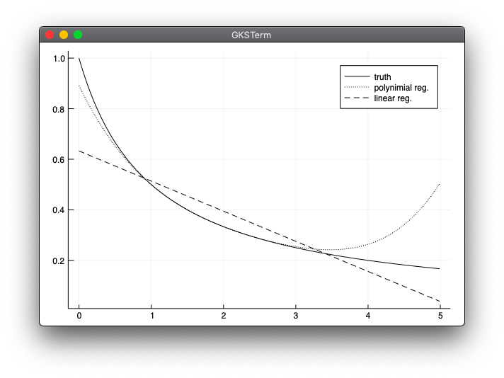
- 本と同じような結果が出て一安心ですが、実はここですごくハマってしまいました。ハマった点は下の方に記載しています。
バイアスとバリアンス
include("polyreg.jl")
using .linearreg
using .polyreg
using Random
using Plots

f(x) = 1 ./ (1 .+ x)

function sample(n)
    x = rand(n) * 5
    y = f(x)
    return x, y
end

xx = collect(0:0.01:4.99)
Random.seed!(0)
y_poly_sum = zeros(length(xx))
y_poly_sum_sq = zeros(length(xx))
y_lin_sum = zeros(length(xx))
y_lin_sum_sq = zeros(length(xx))
y_true = f(xx)
n = 100000
for i in 0:n
    x, y = sample(5)
    poly = polyreg.PolynomialRegression(4)
    polyreg.fit(poly, x, y)
    lin = linearreg.LinearRegression()
    linearreg.fit(lin, x, y)
    y_poly = polyreg.predict(poly, xx)
    global y_poly_sum = y_poly_sum .+ y_poly
    global y_poly_sum_sq = y_poly_sum_sq + (y_poly .- y_true).^2
    y_lin = linearreg.predict(lin, reshape(xx, :, 1))
    global y_lin_sum = y_lin_sum + y_lin
    global y_lin_sum_sq = y_lin_sum_sq + (y_lin .- y_true).^2
end

ax1_1 = plot(xx, (y_lin_sum / n .- y_true).^2, fillrange=(0, (y_lin_sum / n .- y_true).^2), fillcolor=:black, label="bias", title="Linear reg.")
ax1 = plot!(xx, y_lin_sum_sq / n, fillrange=((y_lin_sum / n .- y_true).^2, y_lin_sum_sq / n),fillcolor=:blue, label="variance")

ax1_2 = plot(xx, (y_poly_sum / n .- y_true).^2, fillrange=(0, (y_poly_sum / n .- y_true).^2), fillcolor=:black, label="bias", title="Polynomial reg.")
ax2 = plot!(xx, y_poly_sum_sq / n, fillrange=((y_poly_sum / n .- y_true).^2, y_poly_sum_sq / n), fillcolor=:blue, label="variance")

plot(ax1, ax2, layout=(1,2))
- Pythonの
fill_betweenと同じ書き方が分からず、いろいろ試行錯誤して上記のような書き方になりました。もっと効率のいい書き方があるかもしれません。 -
varianceの所の色は本ではグレーになっていますが、うまく表示できず、blueにしました。
実行結果
実行には第05章02回帰のlinearreg.jlが必要です。
julia> include("bias_var.jl")
WARNING: replacing module linearreg.
WARNING: replacing module polyreg.
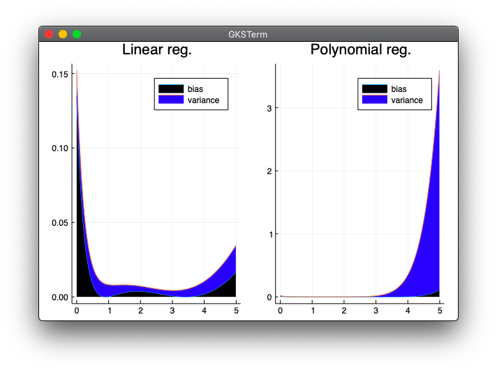
- 本とはY軸の目盛が違いますが、概ね同じ表示が出来ました。
ハマったところ
本のpolyreg.pyでpredictに関しては下記のようになっています。
def predict(self, x):
        r = 0
        for i in range(self.degree + 1):
            r += x**i * self.w_[i]
        return r
Pythonのrangeは0開始です。
>>> for i in range(4):
...     print(i)
...
0
1
2
3
w_[i]で配列のi番目を指定しています。Juliaでは配列のインデックスが1開始なので、下記のように書き換えてしまいました。
 for i in 1:(s.degree + 1)
    r = r .+ x.^i .* s.w_[i]
 end
しかし、本のPythonの場合iが0の時は0乗なのでx**iがx**0となり、1の配列になります。一方、書き換えたJulia版ではfor文の開始を1にしてしまったので、x^iがx^1となってしまいます。渡されるxはcollect(0:0.01:4.99)なので、配列の1番目が$0^1=0$となって、グラフがおかしな表示になってしまいました。下記はその時の実行結果です。
間違った実行結果
julia> include("polyreg_test1.jl")
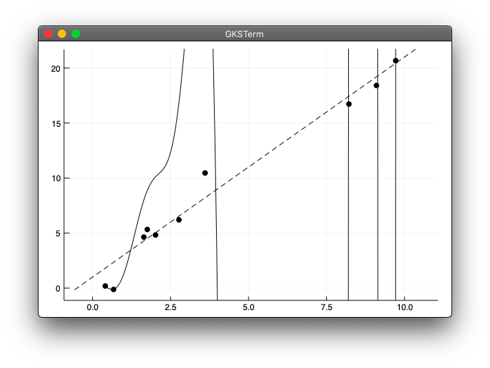
- この時点でそれほどおかしな図ではない気がしたので気づきませんでした。
julia> include("model_mean.jl")
- これで多項式回帰のグラフが
[0, 0]からになっていておかしいことに気づきました。
交差検証
ここはサンプルがないので省略します。