python で複数のvoigt関数にレスポンスいれたフィット
問題背景
複数のフォークト(voigt)関数からなる理論モデルに対して、データから検出器応答やエネルギー分解能を得たい場合がある。特に、X線カロリメータのようなエネルギー分解能のよい検出器をつかって、蛍光X線を計測した場合には、このようなフィットが不可欠であろう。
蛍光X線は、Kα線は1:2の強度でKalpha1とKalpha2の2本が見える。ただし、厳密には、量子状態の計算は単純でなく、結晶分光のようにエネルギー分解能が0.1eV程度まで良い装置で測定したラインを現象論的にあわせ込んだモデルを使う。
Holzer et al., PRA, 56, 6, 1997, 4554-4568 :
これが代表的な論文であり、そこから派生して現象論的なモデルを使っていることが多い。
最近(2016年)の Cu Ka の実測値は
にある。理論計算は、

が最近の計算です。
"shake-off"過程というのは、1s core hole ができるとき、core の電荷の急激な変化により周囲の電子が揺すられて、一緒に複数の電子がイオン化してしまう過程のことです(イオン化せずに励起する場合は"shake-up"と呼びます)。
シリーズ 多電子原子の構造とダイナミックス -独立粒子モデルの来し方行く末- 第6回 原子の電子状態と遷移の計算のために 小池 文博
など詳しく知りたい方は参照ください。
コーディングの方法
コードを読めばわかる人は、google colab 上で動くようにしてますので、
をご覧ください。
- 複数のvoigt関数を全積分した1となるように規格化し、normalizationとgainとエネルギー分解能の3つのみのパラメータとするモデルにする。
- バックグランドはエネルギーEの一次関数で入れる。ただし、一次関数を a + bE のようにすると、Eが大きい場合にフィットの収束が悪くなることがあるので、a + b(E-Eo)のようにbと小さい数の掛け算になるようにする。
- Holzer et al. はローレンチアンの高さ(amplitude)がパラメータとなっている。ローレンチアンは半値幅とamplitudeの掛け算が積分値に比例するので、確率を出す時には注意する。また、ローレンチアンも半値幅と全値幅など適宜が異なる場合があるので、それにも注意が必要。
- モデルが正しくても、初期値がダメだと収束が悪いので、フィットがうまくいかない場合は初期値が変でないことを確認する。
- コピペで同じ絵が再現することを心がけたのでコーディングは冗長です。
- 低エネルギー側のテイルが全くないとわかっている場合は、tail なしでフィットしよう。この例は tail がある場合なので、ない場合は簡単に変更できるはず。
関連記事
pythonでのVoigt関数のプロット方法、フィッティング方法、テイルを入れたフィットをする方法については下記を参照ください。
- pythonでモデルに低エネルギーテイルを入れてフィットする方法
- pythonでパラメータの制限付きでfittingを行う方法
- pythonでフォークト関数(Voigt function)をプロットする方法
- python で直線フィットとガウシアンフィットをする簡単な方法
統計に関して
- xspec の C 統計 : https://heasarc.gsfc.nasa.gov/xanadu/xspec/manual/XSappendixStatistics.html
- ガウス統計とポアソン統計の比較の例 : https://academic.oup.com/pasj/article-abstract/71/4/75/5536242
- 計算方法 : https://link.springer.com/article/10.1007/s10909-014-1098-4
Mn Kalpha の場合
理論モデルのプロット
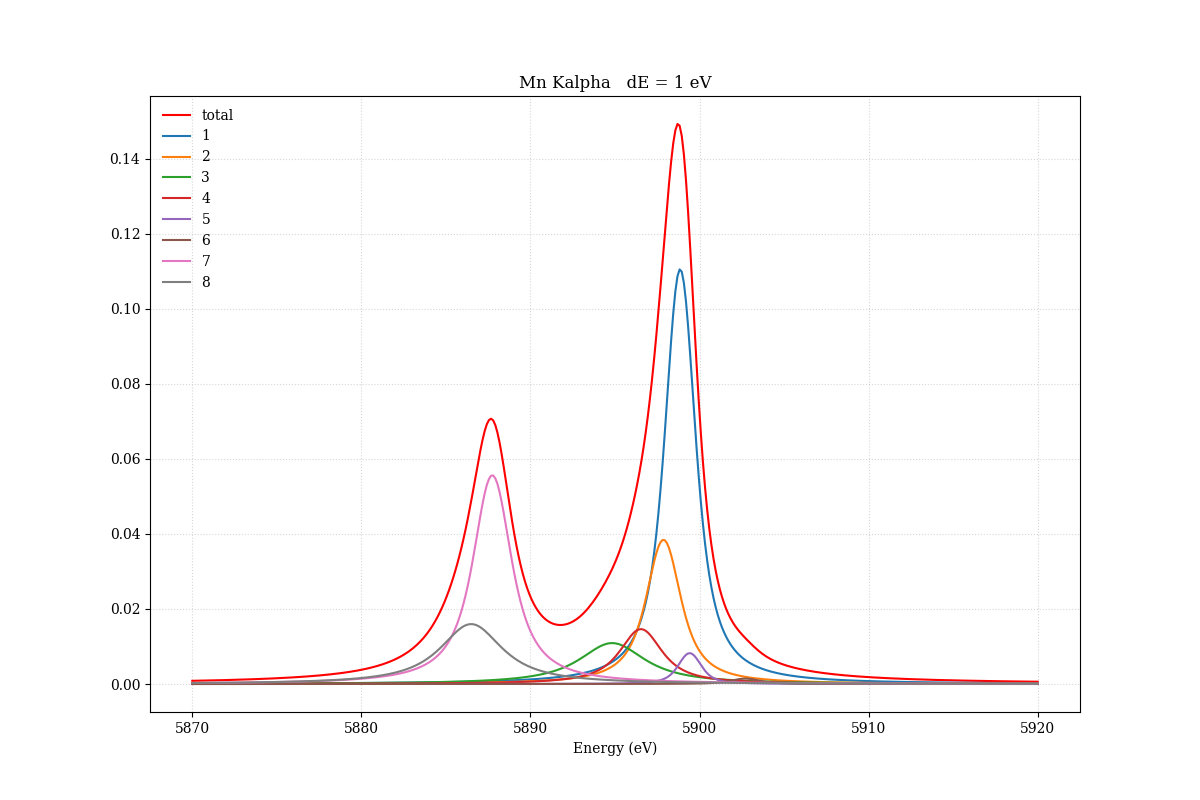
マンガンのK殻からの蛍光X線のモデルはHolzer et al から7本のvoigt関数と、Scott(NASA/GSFC)が現象論的に追加した一本の合計8つのVoigt関数でフィットすることが多い。MnKalha()という関数の中で、voigt()関数を必要数呼び出して足し込んでいる。
MnKalpha()もvoigt()はnormが1の場合に全積分値が1になるように規格化している。
#!/usr/bin/env python
__version__= '1.0'

import matplotlib.pyplot as plt
plt.rcParams['font.family'] = 'serif'
import numpy as np
import scipy as sp
import scipy.special

def MnKalpha(xval,params,consts=[]):
    norm,gw,gain = params
    # norm : normalization
    # gw : sigma of the gaussian
    # gain : if gain changes
    # consttant facter if needed
    # Mn K alpha lines, Holzer, et al., 1997, Phys. Rev. A, 56, 4554, + an emperical addition
    energy = np.array([ 5898.853, 5897.867, 5894.829, 5896.532, 5899.417, 5902.712, 5887.743, 5886.495])
    lgamma =  np.array([    1.715,    2.043,    4.499,    2.663,    0.969,   1.5528,    2.361,    4.216]) # full width at half maximum
    amp =    np.array([    0.790,    0.264,    0.068,    0.096,   0.0714,   0.0106,    0.372,      0.1])
    prob = (amp * lgamma) / np.sum(amp * lgamma) # probabilites for each lines.

    model_y = 0
    if len(consts) == 0:
        consts = np.ones(len(energy))
    else:
        consts = consts

    for i, (ene,lg,pr,con) in enumerate(zip(energy,lgamma,prob,consts)):
        voi = voigt(xval,[ene*gain,lg*0.5,gw])
        model_y += norm * con * pr * voi
    return model_y

def voigt(xval,params):
    center,lw,gw = params
    # center : center of Lorentzian line
    # lw : HWFM of Lorentzian (half-width at half-maximum (HWHM))
    # gw : sigma of the gaussian
    z = (xval - center + 1j*lw)/(gw * np.sqrt(2.0))
    w = scipy.special.wofz(z)
    model_y = (w.real)/(gw * np.sqrt(2.0*np.pi))
    return model_y

x=np.linspace(5870,5920,400)
gfwhm = 1
init_gsigma = gfwhm / 2.35
init_norm = 1.0
init_gain = 1.0

params=[init_norm, init_gsigma, init_gain]
consts = [1,1,1,1,1,1,1,1]

model_MnKalpha = MnKalpha(x,params,consts=consts)

plt.figure(figsize=(12,8))
plt.title("Mn Kalpha   dE = " + str(gfwhm) + " eV")
plt.xlabel("Energy (eV)")
plt.plot(x, model_MnKalpha, 'r-', label = "total")
eye = np.eye(len(consts))
for i, oneeye in enumerate(eye):
    plt.plot(x, MnKalpha(x,params,consts=oneeye), label = str(i+1))
plt.legend(numpoints=1, frameon=False, loc="upper left")
plt.grid(linestyle='dotted',alpha=0.5)
plt.savefig("MnKalpha.png")
plt.show()


plt.figure(figsize=(12,8))
plt.title("Mn Kalpha")
plt.xlabel("Energy (eV)")
eye = np.eye(len(consts))
for de in range(1,10):
    plt.plot(x, MnKalpha(x,[init_norm,de/2.35,1.0],), label = "dE = " + str(de) + " eV (FWHM)")
plt.legend(numpoints=1, frameon=False, loc="upper left")
plt.grid(linestyle='dotted',alpha=0.5)
plt.savefig("MnKalpha_severaldE.png")
plt.show()
Mn Kalpha からの蛍光X線をエネルギー分解能1eV(FWHM)の検出器でなましたスペクトルを示す。マンガンに限らず、Kalpha1とKapha2は強度比がほぼ1:2であることを確認してほしい。
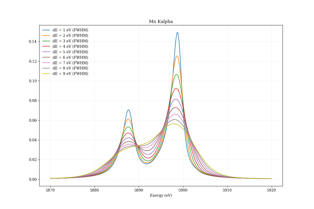
エネルギー分解能を1eVから9eVまで変化させるとこのように変化する。7eVから8eVの間くらいで谷間が見えなくなるので、目でエネルギー分解能を判断するときのひとつの指標になる。
このモデルは、確率分布となるように設定しているため、プロファイルを積分すると1になる。
実データのフィット
超電導遷移端検出器(TES)で得られた実際のMnのスペクトルをフィットしてみよう。データはコード内にベタ書きしているので、任意のデータを使う場合は書き換えてください。
#!/usr/bin/env python
__version__= '1.0'

import matplotlib.pyplot as plt
plt.rcParams['font.family'] = 'serif'
import numpy as np
import scipy as sp
import scipy.optimize as so
import scipy.special

def calcchi(params,consts,model_func,xvalues,yvalues,yerrors):
    model = model_func(xvalues,params,consts)
    chi = (yvalues - model) / yerrors
    return(chi)

# optimizer
def solve_leastsq(xvalues,yvalues,yerrors,param_init,consts,model_func):
    param_output = so.leastsq(
        calcchi,
        param_init,
        args=(consts,model_func, xvalues, yvalues, yerrors),
        full_output=True)
    param_result, covar_output, info, mesg, ier = param_output
    error_result = np.sqrt(covar_output.diagonal())
    dof = len(xvalues) - 1 - len(param_init)
    chi2 = np.sum(np.power(calcchi(param_result,consts,model_func,xvalues,yvalues,yerrors),2.0))
    return([param_result, error_result, chi2, dof])

def mymodel(x,params, consts, tailonly = False):
    norm,gw,gain,P_tailfrac,P_tailtau,bkg1,bkg2 = params
    # norm : nomarlizaion
    # gw : sigma of gaussian
    # gain : gain of the spectrum
    # P_tailfrac : fraction of tail
    # P_tailtau : width of the low energy tail
    # bkg1 : constant of background
    # bkg2 : linearity of background
    initparams = [norm,gw,gain,bkg1,bkg2]
    def rawfunc(x): # local function, updated when mymodel is called
        return MnKalpha(x,initparams,consts=consts)
    model_y = smear(rawfunc, x, P_tailfrac, P_tailtau, tailonly=tailonly)
    return model_y

def MnKalpha(xval,params,consts=[]):
    norm,gw,gain,bkg1,bkg2 = params
    # norm : normalization
    # gw : sigma of the gaussian
    # gain : if gain changes
    # consttant facter if needed
    # Mn K alpha lines, Holzer, et al., 1997, Phys. Rev. A, 56, 4554, + an emperical addition
    energy = np.array([ 5898.853, 5897.867, 5894.829, 5896.532, 5899.417, 5902.712, 5887.743, 5886.495])
    lgamma =  np.array([    1.715,    2.043,    4.499,    2.663,    0.969,   1.5528,    2.361,    4.216]) # full width at half maximum
    amp =    np.array([    0.790,    0.264,    0.068,    0.096,   0.0714,   0.0106,    0.372,      0.1])

    prob = (amp * lgamma) / np.sum(amp * lgamma) # probabilites for each lines.

    model_y = 0
    if len(consts) == 0:
        consts = np.ones(len(energy))
    else:
        consts = consts

    for i, (ene,lg,pr,con) in enumerate(zip(energy,lgamma,prob,consts)):
        voi = voigt(xval,[ene*gain,lg*0.5,gw])
        model_y += norm * con * pr * voi

    background = bkg1 * np.ones(len(xval)) + (xval - np.mean(xval)) * bkg2
    model_y = model_y + background
    # print "bkg1,bkg2 = ", bkg1,bkg2, background
    return model_y

def voigt(xval,params):
    center,lw,gw = params
    # center : center of Lorentzian line
    # lw : HWFM of Lorentzian (half-width at half-maximum (HWHM))
    # gw : sigma of the gaussian
    z = (xval - center + 1j*lw)/(gw * np.sqrt(2.0))
    w = scipy.special.wofz(z)
    model_y = (w.real)/(gw * np.sqrt(2.0*np.pi))
    return model_y

def smear(rawfunc, x, P_tailfrac, P_tailtau, tailonly = False):
    if P_tailfrac <= 1e-5:
        return rawfunc(x)

    dx = x[1] - x[0]
    freq = np.fft.rfftfreq(len(x), d=dx)
    rawspectrum = rawfunc(x)
    ft = np.fft.rfft(rawspectrum)
    if tailonly:
        ft *= P_tailfrac * (1.0 / (1 - 2j * np.pi * freq * P_tailtau) - 0)
    else:
        ft += ft * P_tailfrac * (1.0 / (1 - 2j * np.pi * freq * P_tailtau) - 1)

    smoothspectrum = np.fft.irfft(ft, n=len(x))
    if tailonly:
        pass
    else:
        smoothspectrum[smoothspectrum < 0] = 0
    return smoothspectrum


x = np.linspace(5870.5,5919.5,50)
y = np.array([  42.,   41.,   55.,   40.,   43.,   46.,   69.,   74.,   82., 89.,   85.,   99.,  126.,  149.,  166.,  213.,  252.,  258., 279.,  281.,  243.,  266.,  229.,  254.,  271.,  327.,  390., 398.,  467.,  435.,  387.,  330.,  300.,  215.,  160.,  124., 85.,   79.,   66.,   53.,   46.,   37.,   30.,   45.,   34., 28.,   33.,   35.,   22.,   34.])

yerr = np.sqrt(y)

gfwhm = 6
gw = gfwhm / 2.35
norm = 8000.0
gain = 1.0001
bkg1 = 1.0
bkg2 = 0.0
P_tailfrac = 0.25
P_tailtau = 10
init_params=[norm,gw,gain,P_tailfrac,P_tailtau,bkg1,bkg2]
consts = [1,1,1,1,1,1,1,1]

model_y = mymodel(x,init_params,consts)

plt.figure(figsize=(12,8))
plt.title("Mn Kalpha fit (initial values)")
plt.xlabel("Energy (eV)")
plt.errorbar(x, y, yerr=yerr, fmt='ko', label = "data")
plt.plot(x, model_y, 'r-', label = "model")
plt.legend(numpoints=1, frameon=False, loc="upper left")
plt.grid(linestyle='dotted',alpha=0.5)
plt.savefig("fit_MnKalpha_init.png")
plt.show()

# do fit
result, error, chi2, dof = solve_leastsq(x, y, yerr, init_params, consts, mymodel)

# get results
norm = np.abs(result[0])
norme = np.abs(error[0])

gw = np.abs(result[1])
gwe = np.abs(error[1])

gain = np.abs(result[2])
gaine = np.abs(error[2])

tailfrac = np.abs(result[3])
tailfrac_e = np.abs(error[3])
tailtau = np.abs(result[4])
tailtau_e = np.abs(error[4])

bkg1 = np.abs(result[5])
bkg1e = np.abs(error[5])
bkg2 = np.abs(result[6])
bkg2e = np.abs(error[6])

fwhm = 2.35 * gw
fwhme = 2.35 * gwe

label1 = "N = " + str("%4.2f(+/-%4.2f)" % (norm,norme)) + " g = " + str("%4.2f(+/-%4.2f)" % (gain,gaine)) + " dE = " + str("%4.2f(+/-%4.2f)" % (fwhm,fwhme) + " (FWHM)")
label2 = "tailfrac = " + str("%4.2f(+/-%4.2f)" % (tailfrac,tailfrac_e)) + ", tailtau = " + str("%4.2f(+/-%4.2f)" % (tailtau,tailtau_e))
label3 = "chi/dof = " + str("%4.2f"%chi2) + "/" + str(dof) + " = " + str("%4.2f"%  (chi2/dof))
label4 = "bkg1 = " + str("%4.2f(+/-%4.2f)" % (bkg1,bkg1e)) + " bkg2 = " + str("%4.2f(+/-%4.2f)" % (bkg2,bkg2e))

fitmodel = mymodel(x,result,consts)
plt.figure(figsize=(10,8))
ax1 = plt.subplot2grid((3,1), (0,0), rowspan=2)
plt.title("Mn Kalpha fit : " + label1 + "\n" + label2 + ", " + label3 + "\n" + label4)
#plt.xlabel("Energy (eV)")
plt.errorbar(x, y, yerr=yerr, fmt='ko', label = "data")
plt.plot(x, fitmodel, 'r-', label = "model")
background = bkg1 * np.ones(len(x)) + (x - np.mean(x)) * bkg2
plt.plot(x, background, 'b-', label = "background", alpha = 0.9, lw = 1)
eye = np.eye(len(consts))
for i, oneeye in enumerate(eye):
    plt.plot(x, mymodel(x,result,consts=oneeye), alpha = 0.7, lw = 1, linestyle="--", label = str(i+1))
plt.grid(linestyle='dotted',alpha=0.5)
plt.legend(numpoints=1, frameon=False, loc="upper left")


ax2 = plt.subplot2grid((3,1), (2,0))
plt.xscale('linear')
plt.yscale('linear')
plt.xlabel(r'Energy (eV)')
plt.ylabel(r'Residual')
resi = y - fitmodel
plt.errorbar(x, resi, yerr = yerr, fmt='ko')
plt.legend(numpoints=1, frameon=False, loc="best")
plt.grid(linestyle='dotted',alpha=0.5)
plt.savefig("fit_MnKalpha_result.png")
plt.show()
フィット結果の例はこちら。バックグランドを一次関数で入れている。
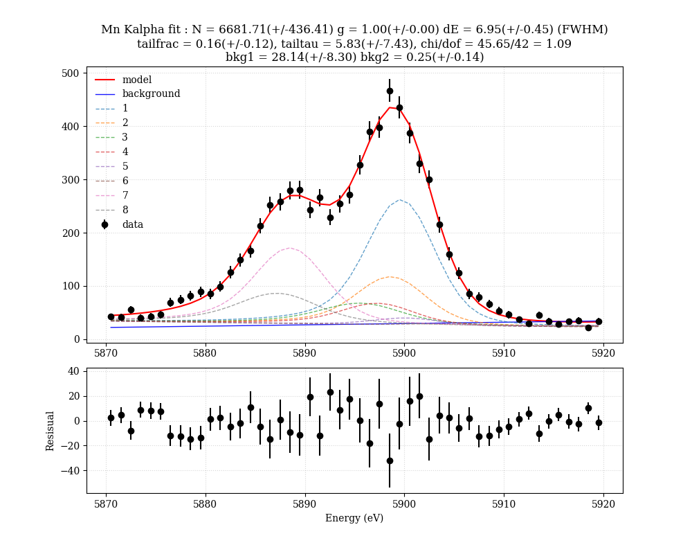
フィットは必ず残差をプロットして、フィットがローカルミニマムに陥ってないか、系統誤差がないか、自分の目で確認しよう。
Fe Kalpha の場合
鉄のKα輝線についても見てみよう。鉄は7つのvoigt関数を使ってフィットする。(chemical effectなので、宇宙の高温プラズマのように鉄がガスの状態の場合は理論どおりの2本だけでよい。)
理論モデルのプロット
#!/usr/bin/env python
__version__= '1.0'

import matplotlib.pyplot as plt
plt.rcParams['font.family'] = 'serif'
import numpy as np
import scipy as sp
import scipy.special

def FeKalpha(xval,params,consts=[]):
    norm,gw,gain = params
    # norm : normalization
    # gw : sigma of the gaussian
    # gain : if gain changes
    # consttant facter if needed
    # Fe K alpha lines, Holzer, et al., 1997, Phys. Rev. A, 56, 4554, + an emperical addition
    energy = np.array([6404.148, 6403.295, 6400.653, 6402.077, 6391.190, 6389.106, 6390.275])
    lgamma = np.array([ 1.613, 1.965, 4.833, 2.803, 2.487, 2.339, 4.433])
    amp = np.array([ 0.697, 0.376, 0.088, 0.136, 0.339, 0.060, 0.102])

    prob = (amp * lgamma) / np.sum(amp * lgamma) # probabilites for each lines.

    model_y = 0
    if len(consts) == 0:
        consts = np.ones(len(energy))
    else:
        consts = consts

    for i, (ene,lg,pr,con) in enumerate(zip(energy,lgamma,prob,consts)):
        voi = voigt(xval,[ene*gain,lg*0.5,gw])
        model_y += norm * con * pr * voi
    return model_y

def voigt(xval,params):
    center,lw,gw = params
    # center : center of Lorentzian line
    # lw : HWFM of Lorentzian (half-width at half-maximum (HWHM))
    # gw : sigma of the gaussian
    z = (xval - center + 1j*lw)/(gw * np.sqrt(2.0))
    w = scipy.special.wofz(z)
    model_y = (w.real)/(gw * np.sqrt(2.0*np.pi))
    return model_y

x=np.linspace(6350,6450,400)
gfwhm = 1
init_gsigma = gfwhm / 2.35
init_norm = 1.0
init_gain = 1.0

params=[init_norm, init_gsigma, init_gain]
consts = [1,1,1,1,1,1,1]

model_FeKalpha = FeKalpha(x,params,consts=consts)

plt.figure(figsize=(12,8))
plt.title("Fe Kalpha   dE = " + str(gfwhm) + " eV")
plt.xlabel("Energy (eV)")
plt.plot(x, model_FeKalpha, 'r-', label = "total")
eye = np.eye(len(consts))
for i, oneeye in enumerate(eye):
    plt.plot(x, FeKalpha(x,params,consts=oneeye), label = str(i+1))
plt.legend(numpoints=1, frameon=False, loc="upper left")
plt.grid(linestyle='dotted',alpha=0.5)
plt.savefig("FeKalpha.png")
plt.show()

plt.figure(figsize=(12,8))
plt.title("Fe Kalpha")
plt.xlabel("Energy (eV)")
eye = np.eye(len(consts))
for de in range(1,10):
    plt.plot(x, FeKalpha(x,[init_norm,de/2.35,1.0],), label = "dE = " + str(de) + " eV (FWHM)")
plt.legend(numpoints=1, frameon=False, loc="upper left")
plt.grid(linestyle='dotted',alpha=0.5)
plt.savefig("FeKalpha_severaldE.png")
plt.show()
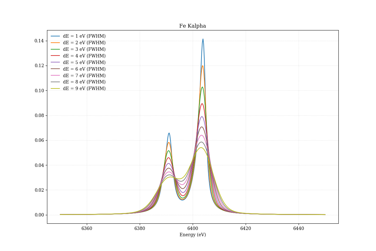
エネルギー分解能 1 eV で見るとこのようになる。
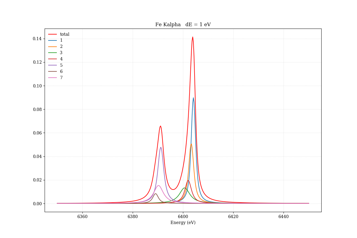
Kalpha1とKalpha2の差の絶対値は大きくなるので、同じ検出器分解能でも谷間は見やすくなることには注意してほしい。
実データのフィット
TESで得られた実際の鉄のK輝線のスペクトルをフィットしてみよう。
#!/usr/bin/env python
__version__= '1.0'

import matplotlib.pyplot as plt
plt.rcParams['font.family'] = 'serif'
import numpy as np
import scipy as sp
import scipy.optimize as so
import scipy.special

def calcchi(params,consts,model_func,xvalues,yvalues,yerrors):
    model = model_func(xvalues,params,consts)
    chi = (yvalues - model) / yerrors
    return(chi)

# optimizer
def solve_leastsq(xvalues,yvalues,yerrors,param_init,consts,model_func):
    param_output = so.leastsq(
        calcchi,
        param_init,
        args=(consts,model_func, xvalues, yvalues, yerrors),
        full_output=True)
    param_result, covar_output, info, mesg, ier = param_output
    error_result = np.sqrt(covar_output.diagonal())
    dof = len(xvalues) - 1 - len(param_init)
    chi2 = np.sum(np.power(calcchi(param_result,consts,model_func,xvalues,yvalues,yerrors),2.0))
    return([param_result, error_result, chi2, dof])

def mymodel(x,params, consts, tailonly = False):
    norm,gw,gain,P_tailfrac,P_tailtau,bkg1,bkg2 = params
    # norm : nomarlizaion
    # gw : sigma of gaussian
    # gain : gain of the spectrum
    # P_tailfrac : fraction of tail
    # P_tailtau : width of the low energy tail
    # bkg1 : constant of background
    # bkg2 : linearity of background
    initparams = [norm,gw,gain,bkg1,bkg2]
    def rawfunc(x): # local function, updated when mymodel is called
        return FeKalpha(x,initparams,consts=consts)
    model_y = smear(rawfunc, x, P_tailfrac, P_tailtau, tailonly=tailonly)
    return model_y

def FeKalpha(xval,params,consts=[]):
    norm,gw,gain,bkg1,bkg2 = params
    # norm : normalization
    # gw : sigma of the gaussian
    # gain : if gain changes
    # consttant facter if needed
    # Fe K alpha lines, Holzer, et al., 1997, Phys. Rev. A, 56, 4554, + an emperical addition
    energy = np.array([6404.148, 6403.295, 6400.653, 6402.077, 6391.190, 6389.106, 6390.275])
    lgamma = np.array([ 1.613, 1.965, 4.833, 2.803, 2.487, 2.339, 4.433])
    amp = np.array([ 0.697, 0.376, 0.088, 0.136, 0.339, 0.060, 0.102])

    prob = (amp * lgamma) / np.sum(amp * lgamma) # probabilites for each lines.

    model_y = 0
    if len(consts) == 0:
        consts = np.ones(len(energy))
    else:
        consts = consts

    for i, (ene,lg,pr,con) in enumerate(zip(energy,lgamma,prob,consts)):
        voi = voigt(xval,[ene*gain,lg*0.5,gw])
        model_y += norm * con * pr * voi

    background = bkg1 * np.ones(len(xval)) + (xval - np.mean(xval)) * bkg2
    model_y = model_y + background
    # print "bkg1,bkg2 = ", bkg1,bkg2, background
    return model_y

def voigt(xval,params):
    center,lw,gw = params
    # center : center of Lorentzian line
    # lw : HWFM of Lorentzian (half-width at half-maximum (HWHM))
    # gw : sigma of the gaussian
    z = (xval - center + 1j*lw)/(gw * np.sqrt(2.0))
    w = scipy.special.wofz(z)
    model_y = (w.real)/(gw * np.sqrt(2.0*np.pi))
    return model_y

def smear(rawfunc, x, P_tailfrac, P_tailtau, tailonly = False):
    if P_tailfrac <= 1e-5:
        return rawfunc(x)

    dx = x[1] - x[0]
    freq = np.fft.rfftfreq(len(x), d=dx)
    rawspectrum = rawfunc(x)
    ft = np.fft.rfft(rawspectrum)
    if tailonly:
        ft *= P_tailfrac * (1.0 / (1 - 2j * np.pi * freq * P_tailtau) - 0)
    else:
        ft += ft * P_tailfrac * (1.0 / (1 - 2j * np.pi * freq * P_tailtau) - 1)

    smoothspectrum = np.fft.irfft(ft, n=len(x))
    if tailonly:
        pass
    else:
        smoothspectrum[smoothspectrum < 0] = 0
    return smoothspectrum


x = np.linspace(6351,6449,99)
y = np.array([ 4,  5,  6,  6,  7,  5,  6,  3,  8,  5, 11,  5,  9,  4,  4,  6, 11, 10, 10,  9,  9, 10, 13,  9,  9, 11, 10,  9, 23, 18, 17, 16, 25, 41, 19, 28, 41, 26, 37, 25, 25, 28, 27, 29, 38, 28, 41, 43, 54, 55, 46, 44, 21, 25, 17, 14,  7, 11, 12, 10,  4,  6,  5,  3,  7,  7,  7,  7, 5,  1,  7,  7,  6,  5,  7,  1,  9,  6,  2,  5,  7,  1,  7,  5,  5, 7,  6,  7,  4,  8,  3,  4,  6,  8,  7,  8, 13,  4,  6])
yerr = np.sqrt(y)

gfwhm = 6
gw = gfwhm / 2.35
norm = 700.0
gain = 0.9995
bkg1 = 1.0
bkg2 = 0.0
P_tailfrac = 0.25
P_tailtau = 10
init_params=[norm,gw,gain,P_tailfrac,P_tailtau,bkg1,bkg2]
consts = [1,1,1,1,1,1,1]

model_y = mymodel(x,init_params,consts)

plt.figure(figsize=(12,8))
plt.title("Fe Kalpha fit (initial values)")
plt.xlabel("Energy (eV)")
plt.errorbar(x, y, yerr=yerr, fmt='ko', label = "data")
plt.plot(x, model_y, 'r-', label = "model")
plt.legend(numpoints=1, frameon=False, loc="upper left")
plt.grid(linestyle='dotted',alpha=0.5)
plt.savefig("fit_FeKalpha_init.png")
plt.show()

# do fit
result, error, chi2, dof = solve_leastsq(x, y, yerr, init_params, consts, mymodel)

# get results
norm = np.abs(result[0])
norme = np.abs(error[0])

gw = np.abs(result[1])
gwe = np.abs(error[1])

gain = np.abs(result[2])
gaine = np.abs(error[2])

tailfrac = np.abs(result[3])
tailfrac_e = np.abs(error[3])
tailtau = np.abs(result[4])
tailtau_e = np.abs(error[4])

bkg1 = np.abs(result[5])
bkg1e = np.abs(error[5])
bkg2 = np.abs(result[6])
bkg2e = np.abs(error[6])

fwhm = 2.35 * gw
fwhme = 2.35 * gwe

label1 = "N = " + str("%4.2f(+/-%4.2f)" % (norm,norme)) + " g = " + str("%4.2f(+/-%4.2f)" % (gain,gaine)) + " dE = " + str("%4.2f(+/-%4.2f)" % (fwhm,fwhme) + " (FWHM)")
label2 = "tailfrac = " + str("%4.2f(+/-%4.2f)" % (tailfrac,tailfrac_e)) + ", tailtau = " + str("%4.2f(+/-%4.2f)" % (tailtau,tailtau_e))
label3 = "chi/dof = " + str("%4.2f"%chi2) + "/" + str(dof) + " = " + str("%4.2f"%  (chi2/dof))
label4 = "bkg1 = " + str("%4.2f(+/-%4.2f)" % (bkg1,bkg1e)) + " bkg2 = " + str("%4.2f(+/-%4.2f)" % (bkg2,bkg2e))

fitmodel = mymodel(x,result,consts)
plt.figure(figsize=(10,8))
ax1 = plt.subplot2grid((3,1), (0,0), rowspan=2)
plt.title("Fe Kalpha fit : " + label1 + "\n" + label2 + ", " + label3 + "\n" + label4)
#plt.xlabel("Energy (eV)")
plt.errorbar(x, y, yerr=yerr, fmt='ko', label = "data")
plt.plot(x, fitmodel, 'r-', label = "model")
background = bkg1 * np.ones(len(x)) + (x - np.mean(x)) * bkg2
plt.plot(x, background, 'b-', label = "background", alpha = 0.9, lw = 1)
eye = np.eye(len(consts))
for i, oneeye in enumerate(eye):
    plt.plot(x, mymodel(x,result,consts=oneeye), alpha = 0.7, lw = 1, linestyle="--", label = str(i+1))
plt.legend(numpoints=1, frameon=False, loc="upper left")
plt.grid(linestyle='dotted',alpha=0.5)

ax2 = plt.subplot2grid((3,1), (2,0))
plt.xscale('linear')
plt.yscale('linear')
plt.xlabel(r'Energy (eV)')
plt.ylabel(r'Residual')
resi = y - fitmodel
plt.errorbar(x, resi, yerr = yerr, fmt='ko')
plt.legend(numpoints=1, frameon=False, loc="best")
plt.grid(linestyle='dotted',alpha=0.5)
plt.savefig("fit_FeKalpha_result.png")
plt.show()
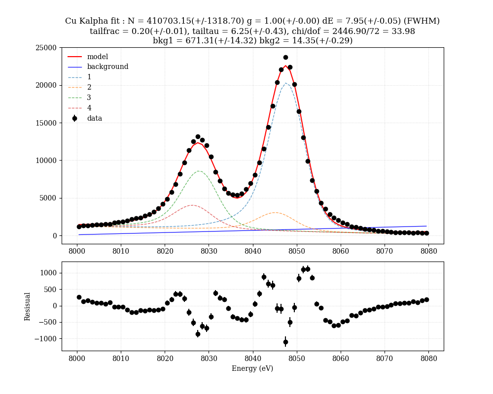
結果がこちら。
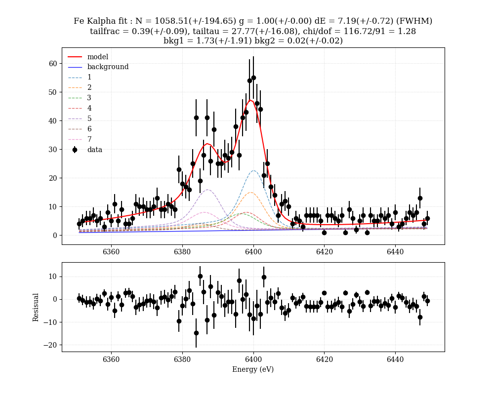
統計が悪い場合は、least squire で最小化する目的関数が異なるので、上記のフィットはガウス統計が成り立つ場合のみであることには注意してほしい。ポアソンが効く場合は下記を参照にしてほしい。
Cu Kalpha の場合
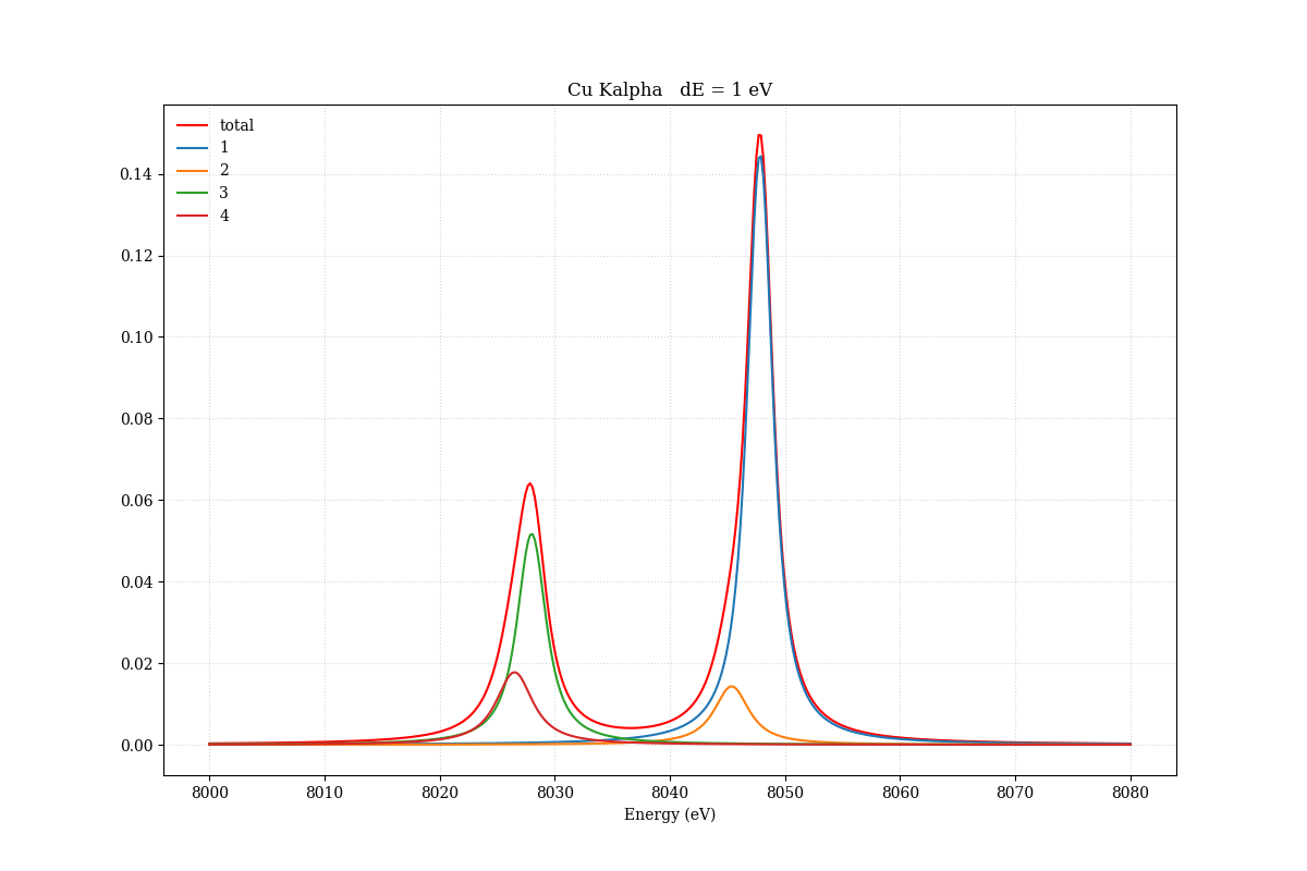
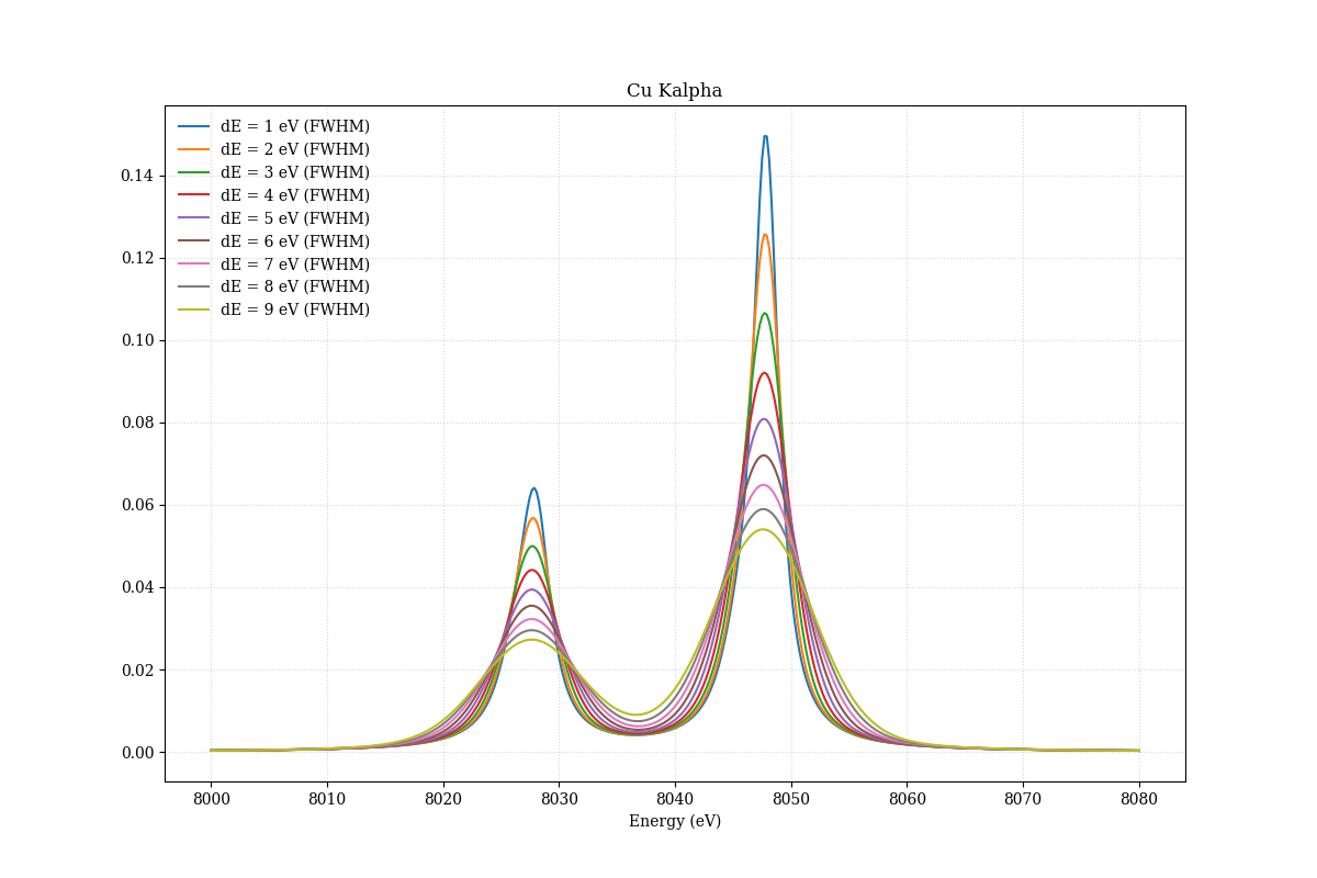
銅のKα輝線についても見てみよう。銅は4つのvoigt関数を使ってフィットする。
理論モデルのプロット
#!/usr/bin/env python
__version__= '1.0'

import matplotlib.pyplot as plt
plt.rcParams['font.family'] = 'serif'
import numpy as np
import scipy as sp
import scipy.special

def CuKalpha(xval,params,consts=[]):
    norm,gw,gain = params
    # norm : normalization
    # gw : sigma of the gaussian
    # gain : if gain changes
    # consttant facter if needed
    # Cu Cu alpha lines, Holzer, et al., 1997, Phys. Rev. A, 56, 4554, + an emperical addition
    energy = np.array([8047.8372, 8045.3672, 8027.9935, 8026.5041])
    lgamma = np.array([2.285, 3.358, 2.667, 3.571])
    amp = np.array([957, 90, 334, 111])

    prob = (amp * lgamma) / np.sum(amp * lgamma) # probabilites for each lines.

    model_y = 0
    if len(consts) == 0:
        consts = np.ones(len(energy))
    else:
        consts = consts

    for i, (ene,lg,pr,con) in enumerate(zip(energy,lgamma,prob,consts)):
        voi = voigt(xval,[ene*gain,lg*0.5,gw])
        model_y += norm * con * pr * voi
    return model_y

def voigt(xval,params):
    center,lw,gw = params
    # center : center of Lorentzian line
    # lw : HWFM of Lorentzian (half-width at half-maximum (HWHM))
    # gw : sigma of the gaussian
    z = (xval - center + 1j*lw)/(gw * np.sqrt(2.0))
    w = scipy.special.wofz(z)
    model_y = (w.real)/(gw * np.sqrt(2.0*np.pi))
    return model_y

x=np.linspace(8000,8080,400)
gfwhm = 1
init_gsigma = gfwhm / 2.35
init_norm = 1.0
init_gain = 1.0

params=[init_norm, init_gsigma, init_gain]
consts = [1,1,1,1]

model_CuKalpha = CuKalpha(x,params,consts=consts)

plt.figure(figsize=(12,8))
plt.title("Cu Kalpha   dE = " + str(gfwhm) + " eV")
plt.xlabel("Energy (eV)")
plt.plot(x, model_CuKalpha, 'r-', label = "total")
eye = np.eye(len(consts))
for i, oneeye in enumerate(eye):
    plt.plot(x, CuKalpha(x,params,consts=oneeye), label = str(i+1))
plt.legend(numpoints=1, frameon=False, loc="upper left")
plt.grid(linestyle='dotted',alpha=0.5)
plt.savefig("CuKalpha.png")
plt.show()

plt.figure(figsize=(12,8))
plt.title("Cu Kalpha")
plt.xlabel("Energy (eV)")
eye = np.eye(len(consts))
for de in range(1,10):
    plt.plot(x, CuKalpha(x,[init_norm,de/2.35,1.0],), label = "dE = " + str(de) + " eV (FWHM)")
plt.legend(numpoints=1, frameon=False, loc="upper left")
plt.grid(linestyle='dotted',alpha=0.5)
plt.savefig("CuKalpha_severaldE.png")
plt.show()
実データのフィット
TESで得られた実際の銅のK輝線のスペクトルをフィットしてみよう。
#!/usr/bin/env python
__version__= '1.0'

import matplotlib.pyplot as plt
plt.rcParams['font.family'] = 'serif'
import numpy as np
import scipy as sp
import scipy.optimize as so
import scipy.special

def calcchi(params,consts,model_func,xvalues,yvalues,yerrors):
    model = model_func(xvalues,params,consts)
    chi = (yvalues - model) / yerrors
    return(chi)

# optimizer
def solve_leastsq(xvalues,yvalues,yerrors,param_init,consts,model_func):
    param_output = so.leastsq(
        calcchi,
        param_init,
        args=(consts,model_func, xvalues, yvalues, yerrors),
        full_output=True)
    param_result, covar_output, info, mesg, ier = param_output
    error_result = np.sqrt(covar_output.diagonal())
    dof = len(xvalues) - 1 - len(param_init)
    chi2 = np.sum(np.power(calcchi(param_result,consts,model_func,xvalues,yvalues,yerrors),2.0))
    return([param_result, error_result, chi2, dof])

def mymodel(x,params, consts, tailonly = False):
    norm,gw,gain,P_tailfrac,P_tailtau,bkg1,bkg2 = params
    # norm : nomarlizaion
    # gw : sigma of gaussian
    # gain : gain of the spectrum
    # P_tailfrac : fraction of tail
    # P_tailtau : width of the low energy tail
    # bkg1 : constant of background
    # bkg2 : linearity of background
    initparams = [norm,gw,gain,bkg1,bkg2]
    def rawfunc(x): # local function, updated when mymodel is called
        return CuKalpha(x,initparams,consts=consts)
    model_y = smear(rawfunc, x, P_tailfrac, P_tailtau, tailonly=tailonly)
    return model_y

def CuKalpha(xval,params,consts=[]):
    norm,gw,gain,bkg1,bkg2 = params
    # norm : normalization
    # gw : sigma of the gaussian
    # gain : if gain changes
    # consttant facter if needed
    # Cu K alpha lines, Holzer, et al., 1997, Phys. Rev. A, 56, 4554, + an emperical addition
    energy = np.array([8047.8372, 8045.3672, 8027.9935, 8026.5041])
    lgamma = np.array([2.285, 3.358, 2.667, 3.571])
    amp = np.array([957, 90, 334, 111])

    prob = (amp * lgamma) / np.sum(amp * lgamma) # probabilites for each lines.

    model_y = 0
    if len(consts) == 0:
        consts = np.ones(len(energy))
    else:
        consts = consts

    for i, (ene,lg,pr,con) in enumerate(zip(energy,lgamma,prob,consts)):
        voi = voigt(xval,[ene*gain,lg*0.5,gw])
        model_y += norm * con * pr * voi

    background = bkg1 * np.ones(len(xval)) + (xval - np.mean(xval)) * bkg2
    model_y = model_y + background
    # print "bkg1,bkg2 = ", bkg1,bkg2, background
    return model_y

def voigt(xval,params):
    center,lw,gw = params
    # center : center of Lorentzian line
    # lw : HWFM of Lorentzian (half-width at half-maximum (HWHM))
    # gw : sigma of the gaussian
    z = (xval - center + 1j*lw)/(gw * np.sqrt(2.0))
    w = scipy.special.wofz(z)
    model_y = (w.real)/(gw * np.sqrt(2.0*np.pi))
    return model_y

def smear(rawfunc, x, P_tailfrac, P_tailtau, tailonly = False):
    if P_tailfrac <= 1e-5:
        return rawfunc(x)

    dx = x[1] - x[0]
    freq = np.fft.rfftfreq(len(x), d=dx)
    rawspectrum = rawfunc(x)
    ft = np.fft.rfft(rawspectrum)
    if tailonly:
        ft *= P_tailfrac * (1.0 / (1 - 2j * np.pi * freq * P_tailtau) - 0)
    else:
        ft += ft * P_tailfrac * (1.0 / (1 - 2j * np.pi * freq * P_tailtau) - 1)

    smoothspectrum = np.fft.irfft(ft, n=len(x))
    if tailonly:
        pass
    else:
        smoothspectrum[smoothspectrum < 0] = 0
    return smoothspectrum


x = np.array([8000.5,8001.5,8002.5,8003.5,8004.5,8005.5,8006.5,8007.5,8008.5,8009.5,8010.5,8011.5,8012.5,8013.5,8014.5,8015.5,8016.5,8017.5,8018.5,8019.5,8020.5,8021.5,8022.5,8023.5,8024.5,8025.5,8026.5,8027.5,8028.5,8029.5,8030.5,8031.5,8032.5,8033.5,8034.5,8035.5,8036.5,8037.5,8038.5,8039.5,8040.5,8041.5,8042.5,8043.5,8044.5,8045.5,8046.5,8047.5,8048.5,8049.5,8050.5,8051.5,8052.5,8053.5,8054.5,8055.5,8056.5,8057.5,8058.5,8059.5,8060.5,8061.5,8062.5,8063.5,8064.5,8065.5,8066.5,8067.5,8068.5,8069.5,8070.5,8071.5,8072.5,8073.5,8074.5,8075.5,8076.5,8077.5,8078.5,8079.5,8080.5,8081.5,8082.5,8083.5,8084.5,8085.5,8086.5,8087.5,8088.5,8089.5,8090.5,8091.5,8092.5,8093.5,8094.5,8095.5,8096.5,8097.5,8098.5,8099.5])
y = np.array([1193,1330,1316,1381,1427,1458,1514,1509,1694,1750,1813,1990,2163,2288,2384,2603,2820,3178,3622,4207,4833,5755,6814,8193,9707,11339,12500,13188,12718,12013,10499,8450,7280,6207,5662,5428,5343,5590,6165,6964,8077,9666,11527,14431,17240,20384,22089,23681,22407,20108,16483,13058,9891,7371,5919,4349,3537,2794,2385,2030,1689,1507,1211,1147,986,843,774,714,617,584,536,469,418,403,385,383,341,369,322,325,290,262,287,272,259,226,192,184,186,135,134,140,122,99,118,87,86,92,87,74])

emin=8000.
emax=8080.
cutid=np.where( (x>emin) & (x<emax))[0]
x = x[cutid]
y = y[cutid]
yerr = np.sqrt(y)

gfwhm = 8
gw = gfwhm / 2.35
norm = 500000.0
gain = 1.0
bkg1 = 1.0
bkg2 = 0.0
P_tailfrac = 0.25
P_tailtau = 10
init_params=[norm,gw,gain,P_tailfrac,P_tailtau,bkg1,bkg2]
consts = [1,1,1,1]

model_y = mymodel(x,init_params,consts)

plt.figure(figsize=(12,8))
plt.title("Cu Kalpha fit (initial values)")
plt.xlabel("Energy (eV)")
plt.errorbar(x, y, yerr=yerr, fmt='ko', label = "data")
plt.plot(x, model_y, 'r-', label = "model")
plt.legend(numpoints=1, frameon=False, loc="upper left")
plt.grid(linestyle='dotted',alpha=0.5)
plt.savefig("fit_CuKalpha_init.png")
plt.show()

# do fit
result, error, chi2, dof = solve_leastsq(x, y, yerr, init_params, consts, mymodel)

# get results
norm = np.abs(result[0])
norme = np.abs(error[0])

gw = np.abs(result[1])
gwe = np.abs(error[1])

gain = np.abs(result[2])
gaine = np.abs(error[2])

tailfrac = np.abs(result[3])
tailfrac_e = np.abs(error[3])
tailtau = np.abs(result[4])
tailtau_e = np.abs(error[4])

bkg1 = np.abs(result[5])
bkg1e = np.abs(error[5])
bkg2 = np.abs(result[6])
bkg2e = np.abs(error[6])

fwhm = 2.35 * gw
fwhme = 2.35 * gwe

label1 = "N = " + str("%4.2f(+/-%4.2f)" % (norm,norme)) + " g = " + str("%4.2f(+/-%4.2f)" % (gain,gaine)) + " dE = " + str("%4.2f(+/-%4.2f)" % (fwhm,fwhme) + " (FWHM)")
label2 = "tailfrac = " + str("%4.2f(+/-%4.2f)" % (tailfrac,tailfrac_e)) + ", tailtau = " + str("%4.2f(+/-%4.2f)" % (tailtau,tailtau_e))
label3 = "chi/dof = " + str("%4.2f"%chi2) + "/" + str(dof) + " = " + str("%4.2f"%  (chi2/dof))
label4 = "bkg1 = " + str("%4.2f(+/-%4.2f)" % (bkg1,bkg1e)) + " bkg2 = " + str("%4.2f(+/-%4.2f)" % (bkg2,bkg2e))

fitmodel = mymodel(x,result,consts)
plt.figure(figsize=(10,8))
ax1 = plt.subplot2grid((3,1), (0,0), rowspan=2)
plt.title("Cu Kalpha fit : " + label1 + "\n" + label2 + ", " + label3 + "\n" + label4)
#plt.xlabel("Energy (eV)")
plt.errorbar(x, y, yerr=yerr, fmt='ko', label = "data")
plt.plot(x, fitmodel, 'r-', label = "model")
background = bkg1 * np.ones(len(x)) + (x - np.mean(x)) * bkg2
plt.plot(x, background, 'b-', label = "background", alpha = 0.9, lw = 1)
eye = np.eye(len(consts))
for i, oneeye in enumerate(eye):
    plt.plot(x, mymodel(x,result,consts=oneeye), alpha = 0.7, lw = 1, linestyle="--", label = str(i+1))
plt.legend(numpoints=1, frameon=False, loc="upper left")
plt.grid(linestyle='dotted',alpha=0.5)

ax2 = plt.subplot2grid((3,1), (2,0))
plt.xscale('linear')
plt.yscale('linear')
plt.xlabel(r'Energy (eV)')
plt.ylabel(r'Resisual')
resi = y - fitmodel
plt.errorbar(x, resi, yerr = yerr, fmt='ko')
plt.legend(numpoints=1, frameon=False, loc="best")
plt.grid(linestyle='dotted',alpha=0.5)
plt.savefig("fit_CuKalpha_result.png")
plt.show()
フィットがうまくいかない場合
下記の googlecolab のリンク先の最後に、フィットがうまくいかない例として一つ挙げています。
具体的には、MnKaの場合で、
gfwhm = 1
# gfwhm = 4
のように、初期のラインの幅をわざと細くしてフィットした場合です。この場合は、scipy の leastsq だとヘッセ行列がゼロになってしまい、逆行列が NaN になってしまうため、エラーが出せずに終了してしまいます。
Both actual and predicted relative reductions in the sum of squares
  are at most 0.000000 and the relative error between two consecutive iterates is at
  most 0.000000
というエラーメッセージがでていて、これは、パラメータを動かしても誤差関数の変化量がゼロだから上手くフィットが進行してないかも?というツッコミになります。
一方、least_squares だと、正しく計算できます。これは多少のアルゴリズムの違いが重要という意味ではなくて、データに対して不適切な初期値を与えてしまうと、パラメータを変えても誤差関数が全く変化しない(パラメータの微分に対して変化量がゼロ)になり、誤差行列が決まらなくなってしまう、ということが本質的で、アルゴリズムは正しいモデルとデータを設定できた後の話になります。なので、フィットが上手くいかない場合は、モデルの自由度をデータから十分に制限できるかどうかを確認しましょう。
関連記事