pythonでパラメータの制限付きでfittingを行う方法

パラメータの制限付きfitting

python で直線フィットとガウシアンフィットをする簡単な方法 では、scipy.optimize.leastsq を用いた簡単なフィット方法を紹介したが、パラメータの制限付きでフィットしたい場合は、scipy.optimize.least_squires を用いる必要がある。基本的な使い方は同じで、bounds に上限値と下限値を入れるだけである。

制限方法

scipy.optimize の least_squares には bounds というオプションがあるので、ここにパラメータの上限と下限の配列を入れるだけである。least_squares は２乗値の最小化問題なので、一般的な最小化問題よりは速く収束する。

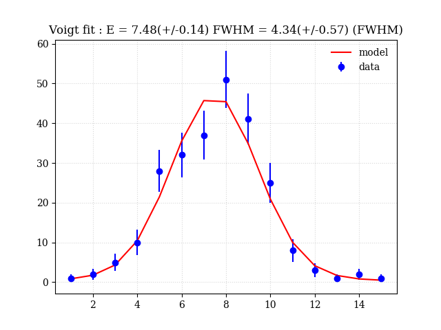
voigt 関数のパラメータ制限付き fitting の例

voigt 関数のフィットの例を使って、パラメータの制限付きフィットの例を示す。
エラーの計算方法がscipy.optimize.leastsq とscipy.optimize.least_squires で若干異なる。

python で voigt 関数をプロット方法は、pythonでフォークト関数(Voigt function)をプロットする方法を参照。

この例では、bounds = [[0, 0, 0, 0],[300, 100, 100, 100]] として、４つのパラメータ(norm,center,lw,gw)を適当に正の範囲で制限する例を示した。

fit_voigt_lq.py

#!/usr/bin/env python

__version__= '1.0'
# This is created from the code made by M.Sawada during SXS tests. 

import matplotlib.pyplot as plt
plt.rcParams['font.family'] = 'serif'
import numpy as np
import scipy as sp
import scipy.optimize as so
import scipy.special

def calcchi(params,consts,model_func,xvalues,yvalues,yerrors):
    model = model_func(xvalues,params,consts)
    chi = (yvalues - model) / yerrors
    return(chi)

# optimizer
def solve_least_squares(xvalues, yvalues, yerrors, param_init, consts, model_func, bounds=(-np.inf, np.inf)):
    param_output = so.least_squares(
        calcchi,
        param_init,
        bounds=bounds,
        args=(consts, model_func, xvalues, yvalues, yerrors))
    param_result = param_output.x
    hessian = np.dot(param_output.jac.T, param_output.jac)
    covar_output = np.array(np.linalg.inv(hessian))
    error_result = np.sqrt(covar_output.diagonal())
    dof = len(xvalues) - 1 - len(param_init)
    chi2 = np.sum(np.power(calcchi(param_result,consts,model_func,xvalues,yvalues,yerrors),2.0))
    return([param_result, error_result, chi2, dof])

# model
def mymodel(xvalues,params,consts):
    norm,center,lw,gw = params
    # norm : normalization 
    # center : center of Lorentzian line
    # lw : HWFM of Lorentzian 
    # gw : sigma of the gaussian 
    c0,c1 = consts
    z = (xvalues - center + 1j*lw)/(gw * np.sqrt(2.0))
    w = scipy.special.wofz(z)
    model_y = norm * (w.real)/(gw * np.sqrt(2.0*np.pi))
    return model_y

# set data
x = np.array([ 1, 2, 3,  4,  5, 6,   7,  8,  9, 10, 11, 12, 13, 14, 15])
y = np.array([ 1, 2, 5, 10, 28, 32, 37, 51, 41, 25,  8,  3,  1,  2,  1])

# initialize parameter 
norm_init = 60.
lorent_init = 2.
gauss_sigma_init = 2.
init_params = np.array([norm_init, np.median(x), lorent_init, gauss_sigma_init])
# initialize constants 
consts = np.array([0,0]) 
bounds = [[0, 0, 0, 0],
         [300, 100, 100, 100]]

# do fit 
result, error, chi2, dof = solve_least_squares(x, y, np.sqrt(y), init_params, consts, mymodel, bounds)

# get results 
ene = result[1]
lw = np.abs(result[2])
gw = np.abs(result[3])

enee = error[1]
lwe = np.abs(error[2])
gwe = np.abs(error[3])

fwhm = 2.35 * gw
fwhme = 2.35 * gwe

label = "E = " + str("%4.2f(+/-%4.2f)" % (ene,enee)) + " FWHM = " + str("%4.2f(+/-%4.2f)" % (fwhm,fwhme) + " (FWHM)")
print(label)

# plot results
plt.title("Voigt fit : " + label)
model_y = mymodel(x,result,consts)
plt.errorbar(x, y, yerr = np.sqrt(y), fmt="bo", label = "data")
plt.plot(x, model_y, 'r-', label = "model")
plt.legend(numpoints=1, frameon=False, loc="best")
plt.grid(linestyle='dotted',alpha=0.5)

plt.savefig("voigtfit_lq.png")
plt.show()

生成される図はこちら。

一般的な注意

パラメータに制限をつけると、計算が遅くなったり、変な値に収束することも多い。本当に制限すべきパラメータなのか、データからそもそも制限できないパラメータをフリーにしてないか、あるいは何らかの方法でパラメータを固定できないのかをよく考えた上で、必要な場合のみ制限をつけよう。