python でテイルを入れてモデルフィットする方法
pythonで取得したデータをモデルフィットしたい場合で、検出器応用による非対称成分(e.g., low energy tail)や、簡易的な検出器応答を入れてフィットしたい場合は、
モデル(ガウス関数、voigt関数)に対して、検出器応答を畳み込んでから、データとモデルフィットを行う必要がある。
簡単な検出器応答であれば、FFTの畳み込みを使って高速で実装が可能である。ここでは、python で voigt 関数に対して、FFTの畳み込みを用いて low energy tail を入れる例を、テーブルモデルの場合(時間空間でモデルを生成しFFTする場合)と周波数空間で関数を入れる方法の2つを示す。
実際の応用例はこちら
- Absolute Energy Calibration of X-ray TESs with 0.04 eV Uncertainty at 6.4 keV in a Hadron-Beam Environment, H. Tatsuno et al.,
python で low energy tail を入れる方法
テーブルを用いてたたみ込む場合はsmear_table_expを用いる。smear_mass は、one-sided exponential の FFT を使った例である。
サンプルコード
#!/usr/bin/env python
__version__= '1.0'
import matplotlib.pyplot as plt
plt.rcParams['font.family'] = 'serif'
import numpy as np
import scipy as sp
import scipy.special
def voigt(xval,params):
norm,center,lw,gw = params
# norm : normalization
# center : center of Lorentzian line
# lw : HWFM of Lorentzian
# gw : sigma of the gaussian
z = (xval - center + 1j*lw)/(gw * np.sqrt(2.0))
w = scipy.special.wofz(z)
model_y = norm * (w.real)/(gw * np.sqrt(2.0*np.pi))
return model_y
# resp という検出器応答関数を受け取り、FFTする。
def smear_table_exp(rawfunc, resp, x, P_resolution, P_tailfrac, P_tailtau, tailonly = False):
dx = x[1] - x[0]
freq = np.fft.fftfreq(len(x), d=dx)
rawspectrum = rawfunc(x)
ft = np.fft.fft(rawspectrum)
ft_resp = np.fft.fft(resp)
if tailonly:
gt = ft * ft_resp
else:
gt = ft * ft_resp + (1-P_tailfrac) * ft
smoothspectrum = np.fft.ifft(gt, n=len(x))
smoothspectrum[smoothspectrum < 0] = 0
return smoothspectrum
# one-sided exponential をFFTした関数を周波数空間で用いる。
def smear_mass(rawfunc, x, P_resolution, P_tailfrac, P_tailtau, tailonly = False):
if P_tailfrac <= 1e-5:
return rawfunc(x)
dx = x[1] - x[0]
freq = np.fft.rfftfreq(len(x), d=dx)
rawspectrum = rawfunc(x)
ft = np.fft.rfft(rawspectrum)
if tailonly:
ft *= P_tailfrac * (1.0 / (1 - 2j * np.pi * freq * P_tailtau) - 0)
else:
ft += ft * P_tailfrac * (1.0 / (1 - 2j * np.pi * freq * P_tailtau) - 1)
smoothspectrum = np.fft.irfft(ft, n=len(x))
if tailonly:
pass
else:
smoothspectrum[smoothspectrum < 0] = 0
return smoothspectrum
P_gaussfwhm = 5
P_tailtau = 10
P_resolution = 3
P_tailfrac = 0.4
# plot init function
x = np.arange(0,100,0.1)
xc = np.mean(x)
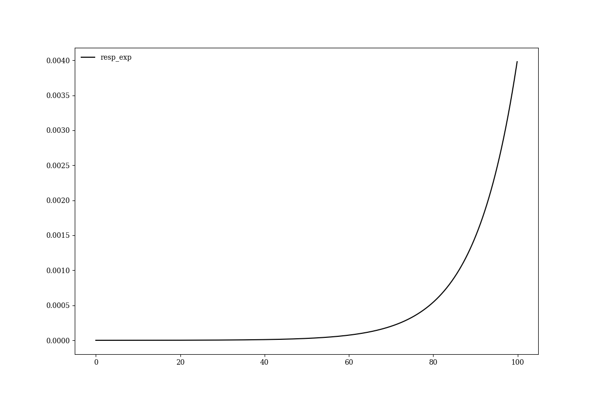
resp_exp = np.exp((x)/P_tailtau)
resp_exp = P_tailfrac * resp_exp/np.sum(resp_exp)
plt.figure(figsize=(12,8))
plt.plot(x, resp_exp, 'k-', label = "resp_exp")
plt.legend(numpoints=1, frameon=False, loc="upper left")
plt.savefig("comp_resp.png")
plt.show()
initparams = [1,xc,1,1]
def rawfunc(x):
return voigt(x,initparams)
sexp = smear_table_exp(rawfunc, resp_exp, x, P_resolution, P_tailfrac, P_tailtau)
sout = smear_mass(rawfunc, x, P_resolution, P_tailfrac, P_tailtau)
tail = smear_mass(rawfunc, x, P_resolution, P_tailfrac, P_tailtau, tailonly=True)
plt.figure(figsize=(12,8))
plt.title("Voigt function with LE tail")
plt.plot(x, sout, 'r-', label = "smeard : a="+str("%3.3e" % np.sum(sout)))
plt.plot(x, tail, 'r--', label = "tail only: a="+str("%3.3e" % np.sum(tail)))
plt.plot(x, sexp, 'b--', label = "resp table exp a="+str("%3.3e" % np.sum(sexp)))
plt.legend(numpoints=1, frameon=False, loc="upper left")
plt.grid(linestyle='dotted',alpha=0.5)
plt.savefig("lwtail_comp_spec.png")
plt.show()
実行結果
時系列で one-sided exponentialのフィルターを用いる。
これをFFTして、フーリエ空間で掛け算を行う。one-sided exponential の FFT は解析的に出せるので、それをつかってフーリエフィルターをかける例でも試し、両者を比較した。
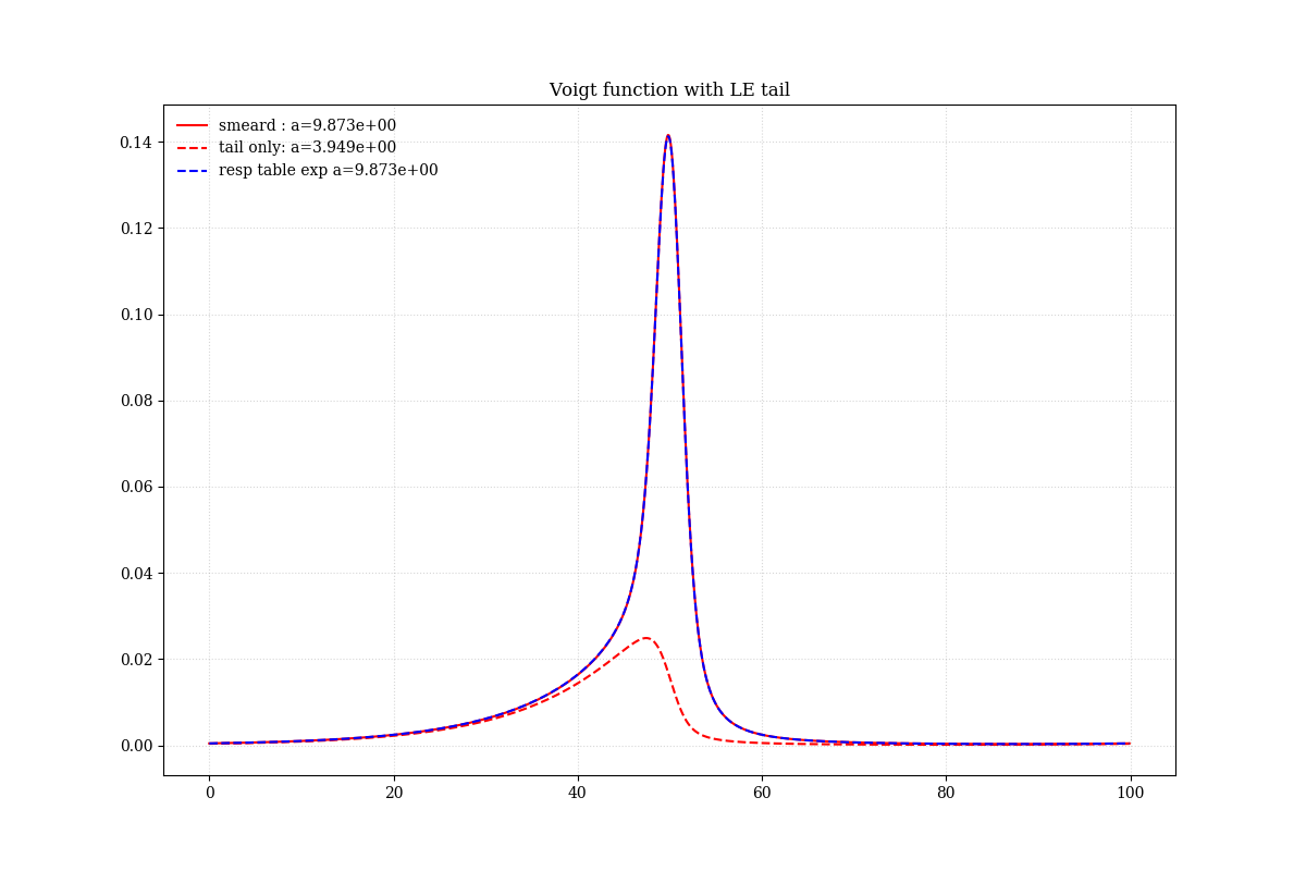
結果はどちらも同じように、low energy 側に tail を生成することができる。
python で low energy tail を入れてfittingする方法
モデルが作れたら、フィットするにはパラメータが更新するたびにモデルを更新できるようにすればOKである。mymodel関数はパラメータの更新ごとに呼び出され、そのためローカルに定義される rawfunc が必要になる。
サンプルコード
#!/usr/bin/env python
__version__= '1.0'
import matplotlib.pyplot as plt
plt.rcParams['font.family'] = 'serif'
import numpy as np
import scipy as sp
import scipy.optimize as so
import scipy.special
def calcchi(params,consts,model_func,xvalues,yvalues,yerrors):
model = model_func(xvalues,params,consts)
chi = (yvalues - model) / yerrors
return(chi)
# optimizer
def solve_leastsq(xvalues,yvalues,yerrors,param_init,consts,model_func):
param_output = so.leastsq(
calcchi,
param_init,
args=(consts,model_func, xvalues, yvalues, yerrors),
full_output=True)
param_result, covar_output, info, mesg, ier = param_output
error_result = np.sqrt(covar_output.diagonal())
dof = len(xvalues) - 1 - len(param_init)
chi2 = np.sum(np.power(calcchi(param_result,consts,model_func,xvalues,yvalues,yerrors),2.0))
return([param_result, error_result, chi2, dof])
def mymodel(x,params, consts, tailonly = False):
norm,center,lw,gw, P_tailfrac, P_tailtau = params
initparams = [norm,center,lw,gw]
def rawfunc(x): # local function, updated when mymodel is called
return voigt(x,initparams)
model_y = smear(rawfunc, x, P_tailfrac, P_tailtau, tailonly=tailonly)
return model_y
def voigt(xval,params,consts=None):
norm,center,lw,gw = params
# norm : normalization
# center : center of Lorentzian line
# lw : HWFM of Lorentzian
# gw : sigma of the gaussian
z = (xval - center + 1j*lw)/(gw * np.sqrt(2.0))
w = scipy.special.wofz(z)
model_y = norm * (w.real)/(gw * np.sqrt(2.0*np.pi))
return model_y
def smear(rawfunc, x, P_tailfrac, P_tailtau, tailonly = False):
if P_tailfrac <= 1e-5: # skip when tail fraction is too small
return rawfunc(x)
dx = x[1] - x[0]
freq = np.fft.rfftfreq(len(x), d=dx)
rawspectrum = rawfunc(x)
ft = np.fft.rfft(rawspectrum)
# a tail is defined in FFT of one-sided exponetial = P_tailfrac x exp(-E/P_tailtau)
if tailonly:
ft *= P_tailfrac * (1.0 / (1 - 2j * np.pi * freq * P_tailtau) - 0)
else:
ft += ft * P_tailfrac * (1.0 / (1 - 2j * np.pi * freq * P_tailtau) - 1)
smoothspectrum = np.fft.irfft(ft, n=len(x))
if tailonly:
pass
else: # a count spectrum is assumed, so a negative value is avoided
smoothspectrum[smoothspectrum < 0] = 0 #
return smoothspectrum
# set data
x = np.array([ 1, 2, 3, 4, 5, 6, 7, 8, 9, 10, 11, 12, 13, 14, 15, 16, 17, 18, 19, 20, 21, 22, 23, 24, 25],dtype='float')
y = np.array([ 1, 3, 2, 4, 7, 5, 11, 8, 10, 9, 11, 12, 17, 21, 35, 45, 69, 78, 62, 52, 33, 21, 10, 6, 1],dtype='float')
# initialize parameter
norm_init = 400.
lorent_init = 1.
gauss_sigma_init = 1.
P_tailfrac = 0.25
P_tailtau = 10
init_params = [norm_init, x[np.argmax(y)], lorent_init, gauss_sigma_init, P_tailfrac, P_tailtau]
init_params = np.array(init_params)
print "init_params = ", init_params
consts = np.array([0,0]) # not used for now
# generete initisal functions
model_y = mymodel(x,init_params,consts)
model_y_tailonly = mymodel(x,init_params,consts, tailonly = True)
# check plot results of initial settings
plt.title("Voigt fit : check init ")
print "modey_y = ", model_y
plt.errorbar(x, y, yerr = np.sqrt(y), fmt="bo", label = "data")
plt.plot(x, model_y, 'r-', label = "model")
plt.plot(x, model_y_tailonly, 'r--', label = "model(tail)")
plt.legend(numpoints=1, frameon=False, loc="best")
plt.grid(linestyle='dotted',alpha=0.5)
plt.savefig("check_init_voigtfit_wtail.png")
plt.show()
# do fit
result, error, chi2, dof = solve_leastsq(x, y, np.sqrt(y), init_params, consts, mymodel)
# get results
ene = result[1]
lw = np.abs(result[2])
gw = np.abs(result[3])
enee = error[1]
lwe = np.abs(error[2])
gwe = np.abs(error[3])
tailfrac = np.abs(result[4])
tailfrac_e = np.abs(error[4])
tailtau = np.abs(result[5])
tailtau_e = np.abs(error[5])
fwhm = 2.35 * gw
fwhme = 2.35 * gwe
label1 = "E = " + str("%4.2f(+/-%4.2f)" % (ene,enee)) + " FWHM = " + str("%4.2f(+/-%4.2f)" % (fwhm,fwhme) + " (FWHM)")
label2 = "tailfrac = " + str("%4.2f(+/-%4.2f)" % (tailfrac,tailfrac_e)) + ", tailtau = " + str("%4.2f(+/-%4.2f)" % (tailtau,tailtau_e))
print(label1)
print(label2)
# plot results
plt.figure(figsize=(12,8))
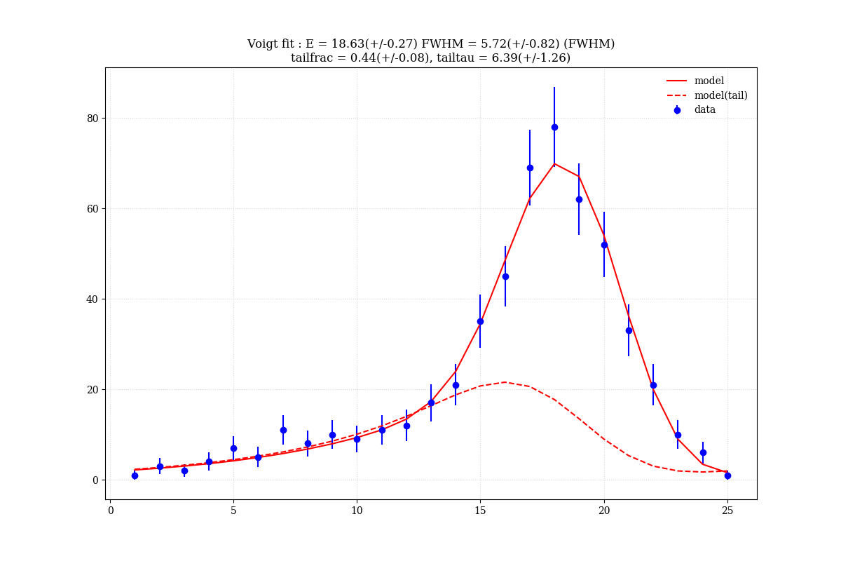
plt.title("Voigt fit : " + label1 + "\n" + label2)
model_y = mymodel(x,result,consts)
model_y_tailonly = mymodel(x,result,consts, tailonly = True)
plt.errorbar(x, y, yerr = np.sqrt(y), fmt="bo", label = "data")
plt.plot(x, model_y, 'r-', label = "model")
plt.plot(x, model_y_tailonly, 'r--', label = "model(tail)")
plt.legend(numpoints=1, frameon=False, loc="best")
plt.grid(linestyle='dotted',alpha=0.5)
plt.savefig("voigtfit_wtail.png")
plt.show()
実行結果
青でデータ点、赤線でモデル、赤点線で low energy tail 成分を表示した。
複雑なフィット
より複雑な場合、とくに現象論的に金属の鉄やマンガンからの蛍光X線のフィットをする場合は、7個や8個もVoigt関数をいれてテイルが必要なことも多い。そのような場合は、
を参照されたい。