「ゼロから作るDeep Learning」(斎藤 康毅 著 オライリー・ジャパン刊)を読んでいる時に、参照したサイト等をメモしていきます。 その7← →その9
5章 誤差逆転伝播法を読んでも、正直、わかったようなわからないような
ただ、この手法によって、勾配の計算が非常に速くなるということ、
「レイヤ」としてモジュール化して実装することの利点くらいは理解しました。
P162からは、誤差逆伝播法を使った学習のプログラムが載っていますが、これを実行するためにはP142以降に載っている、各種定義をしているプログラムも必要です。
6章では、ここまでくる途中で、これってどうするんだろ? と思ったことにも説明してくれているのですが・・・
説明してもらったからと言って、理解できるものではない。
こういう時は、わかることだけ押さえて先に進むか、本の内容に関することは何でもいいから、いろいろやってみるしかないわけで・・・
とりあえず、P169の図を描いてみた。
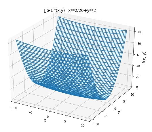
from mpl_toolkits.mplot3d import Axes3D
import matplotlib.pyplot as plt
import numpy as np

def function_2(x, y):
    return x**2/20 + y**2

# x,y の座標範囲
x = np.arange(-10.0, 10.0, 0.1)
y = np.arange(-10.0, 10.0, 0.1)
# x,y の格子データ
X, Y = np.meshgrid(x, y)
# 定義した関数の値をセット
Z = function_2(X, Y)

# Figureを追加
fig = plt.figure(figsize=(10.0, 8.0))
# 3次元の軸を作成
ax = fig.add_subplot(111, projection='3d')
# 軸ラベルを設定
ax.set_title("図6-1 f(x,y)=x**2/20+y**2", size = 14)
ax.set_xlabel("x", size = 14)
ax.set_ylabel("y", size = 14)
ax.set_zlabel("f(x, y)", size = 14)
# 軸目盛を設定
ax.set_xticks([-10.0, -5.0, 0.0, 5.0, 10.0])
ax.set_yticks([-10.0, -5.0, 0.0, 5.0, 10.0])
ax.set_zticks([0.0, 20.0, 40.0, 60.0, 80.0, 100.0])
# 描画
ax.plot_wireframe(X, Y, Z)
# ax.plot_surface(X, Y, Z, rstride=1, cstride=1)
# ax.contour3D(X,Y,Z)
# ax.contourf3D(X,Y,Z)
# ax.scatter3D(np.ravel(X),np.ravel(Y),np.ravel(Z))
plt.show()
plot_wireframe のところを変えると、違う描画になります。
いろいろ調べてるうちに、こんなものもあった。描画したグラフを回転させていろんな方向から見る事ができます。
import numpy as np
import matplotlib
# matplotlib のbackend を設定しているらしいのですが、どういう意味かわかってません。
# ただ、この行を追加したら、グラフを別ウィンドウで開くようになりました。
matplotlib.use('TkAgg')

# for plotting
import matplotlib.pyplot as plt
from mpl_toolkits.mplot3d import Axes3D

def function_2(x, y):
    return x**2/20 + y**2

x = np.arange(-10.0, 10.0, 0.1)
y = np.arange(-10.0, 10.0, 0.1)

X, Y = np.meshgrid(x, y)
Z = function_2(X, Y)

fig = plt.figure()
ax = fig.add_subplot(111, projection='3d')
surf = ax.plot_surface(X, Y, Z, cmap='bwr', linewidth=0)
fig.colorbar(surf)
ax.set_title("Surface Plot")
fig.show()
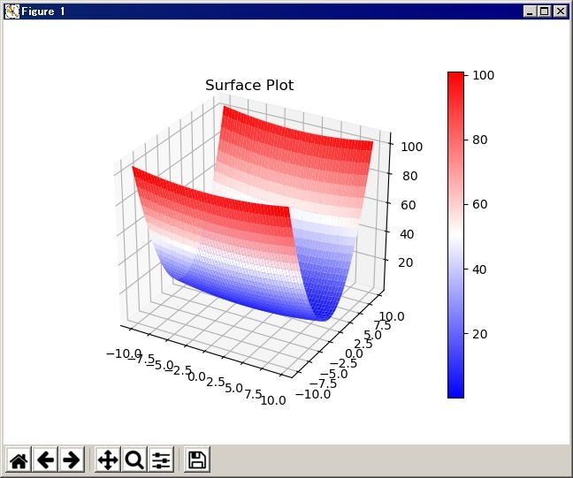
グラフの色は cmap のパラメータで指定するようです。
matplotlib color example code
等高線のほうは、こんな感じで
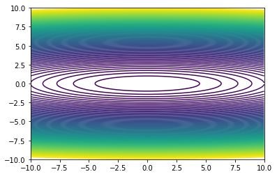
import matplotlib.pyplot as plt
import numpy as np

def function_2(x, y):
    return x**2/20 + y**2

x = np.arange(-10.0, 10.0, 0.1)
y = np.arange(-10.0, 10.0, 0.1)
h = np.arange(0., 100.0, 1.0)
X, Y = np.meshgrid(x, y)
Z = function_2(X, Y)

plt.figure()
plt.contour(X, Y, Z, levels=h)
plt.xlim([-10, 10])
plt.ylim([-10, 10])
plt.show()
contour(x 軸上の位置、y 軸上の位置、座標上での高さ、levels=[線をプロットする高さを指定])
配列x、y の値の刻みを0.1にしているので、線がなめらかですが、表示に時間がかかります。これを1.0にすれば、すぐに表示されますが、線がデコボコです。
h には、線を引きたい高さを指定します。例では、0から100まで、1ずつ線を引いてます。
勾配のベクトル図
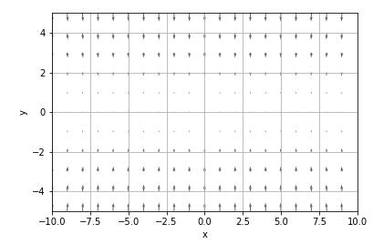
import matplotlib.pyplot as plt
import numpy as np

def _numerical_gradient_no_batch(f, x):
    h = 1e-4  # 0.0001
    grad = np.zeros_like(x)

    for idx in range(x.size):
        tmp_val = x[idx]
        x[idx] = float(tmp_val) + h
        fxh1 = f(x)  # f(x+h)

        x[idx] = tmp_val - h
        fxh2 = f(x)  # f(x-h)
        grad[idx] = (fxh1 - fxh2) / (2*h)

        x[idx] = tmp_val  # 値を元に戻す
    return grad

def numerical_gradient(f, X):
    if X.ndim == 1:
        return _numerical_gradient_no_batch(f, X)
    else:
        grad = np.zeros_like(X)
        for idx, x in enumerate(X):
            grad[idx] = _numerical_gradient_no_batch(f, x)
        return grad

def function_2(x):
    return (x[0]**2/20+x[1]**2)

x = np.arange(-10.0, 10.0, 1.)
y = np.arange(-10.0, 10.0, 1.)
h = np.arange(0., 100.0, 10.0)
X, Y = np.meshgrid(x, y)

X = X.flatten()
Y = Y.flatten()
grad = numerical_gradient(function_2, np.array([X, Y]).T).T

plt.figure()
plt.quiver(X, Y, -grad[0], -grad[1],  angles="xy",color="#666666")
plt.xlim([-10, 10])
plt.ylim([-5, 5])
plt.xlabel('x')
plt.ylabel('y')
plt.grid()
plt.draw()
plt.show()
フォルダch04の gradient_2d.py の function_2 を変えただけです。
quiver (x 軸上の位置、y 軸上の位置、x 軸方向の勾配、y 軸方向の勾配)
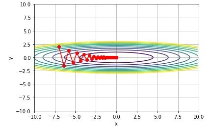
最適化の更新経路の図
import matplotlib.pyplot as plt
import numpy as np

def numerical_gradient(f, x):
    h = 1e-4 # 0.0001
    grad = np.zeros_like(x)

    it = np.nditer(x, flags=['multi_index'], op_flags=['readwrite'])
    while not it.finished:
        idx = it.multi_index
        tmp_val = x[idx]
        x[idx] = tmp_val + h
        fxh1 = f(x) # f(x+h)

        x[idx] = tmp_val - h
        fxh2 = f(x) # f(x-h)
        grad[idx] = (fxh1 - fxh2) / (2*h)

        x[idx] = tmp_val # 値を元に戻す
        it.iternext()

    return grad

def  adagrad(x, lr, grad, v, moment):
    v += grad * grad
    x -= lr * grad / (np.sqrt(v) + 1e-7)
    return x, v

def  momentum(x, lr, grad, v, moment):
    v = moment*v - lr*grad
    x += v
    return x, v

def sgd(x, lr, grad, v = None, moment = None):
    x -= lr * grad
    return x, v

def gradient_descent(opt, f, init_x, lr=0.01, step_num=100, moment=0.9):
    x = init_x
    x_history = []
    v = 0
    for i in range(step_num):
        x_history.append( x.copy() )
        grad = numerical_gradient(f, x)
        x, v = opt(x, lr, grad, v, moment)
    return np.array(x_history)

def function_1(x, y):
    return x**2/20 + y**2

def function_2(x):
    return (x[0]**2/20+x[1]**2)

x = np.arange(-10.0, 10.0, 0.1)
y = np.arange(-10.0, 10.0, 0.1)
h = np.arange(0., 10.0, 1.0)
X, Y = np.meshgrid(x, y)
Z = function_1(X, Y)

plt.figure()
plt.contour(X, Y, Z, levels=h)

init_x = np.array([-7.0, 2.0])
x_history = gradient_descent(sgd, function_2, init_x, lr=0.9, step_num=100)
# x_history = gradient_descent(momentum, function_2, init_x, lr=0.2, step_num=20, moment=0.9)
# x_history = gradient_descent(adagrad, function_2, init_x, lr=0.9, step_num=100)

plt.plot(x_history[:,0], x_history[:,1],'-ro')
plt.xlim([-10, 10])
plt.ylim([-10, 10])
plt.xlabel('x')
plt.ylabel('y')
plt.grid()
plt.show()
SGDの場合、学習係数lr をうまく設定しないと、例のようなジグザグになりません。
1.0だとジグザグにはなりますが、0に収束していきません。
0.7以下だと、ジグザグが目立つ前に0に収束してしまいます。
0.9が一番、それらしいグラフになりました。
momentumの場合は、学習係数lrだけでなく、momentの値を調整しないと、本の例のようになりません。
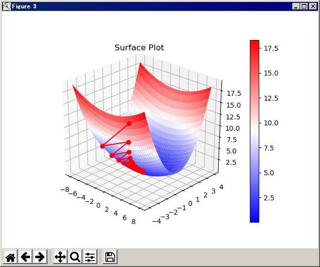
最適化の更新経路の図 3D
import numpy as np
import matplotlib
matplotlib.use('TkAgg')

def numerical_gradient(f, x):
    h = 1e-4 # 0.0001
    grad = np.zeros_like(x)

    it = np.nditer(x, flags=['multi_index'], op_flags=['readwrite'])
    while not it.finished:
        idx = it.multi_index
        tmp_val = x[idx]
        x[idx] = tmp_val + h
        fxh1 = f(x) # f(x+h)

        x[idx] = tmp_val - h
        fxh2 = f(x) # f(x-h)
        grad[idx] = (fxh1 - fxh2) / (2*h)

        x[idx] = tmp_val # 値を元に戻す
        it.iternext()

    return grad

def  adagrad(x, lr, grad, v, moment):
    v += grad * grad
    x -= lr * grad / (np.sqrt(v) + 1e-7)
    return x, v

def  momentum(x, lr, grad, v, moment):
    v = moment*v - lr*grad
    x += v
    return x, v

def sgd(x, lr, grad, v = None, moment = None):
    x -= lr * grad
    return x, v

def gradient_descent(opt, f, init_x, lr=0.01, step_num=100, moment=0.9):
    x = init_x
    x_history = []
    v = 0
    for i in range(step_num):
        w = x.tolist()
        z = f(x)
        w.append(z)
        x_history.append( w )
        grad = numerical_gradient(f, x)
        x, v = opt(x, lr, grad, v, moment)
    return np.array(x_history)

def function_1(x, y):
    return x**2/20 + y**2

def function_2(x):
    return (x[0]**2/20+x[1]**2)


# for plotting
import matplotlib.pyplot as plt
from mpl_toolkits.mplot3d import Axes3D

x = np.arange(-8.0, 8.0, .1)
y = np.arange(-4.0, 4.0, .1)

X, Y = np.meshgrid(x, y)
Z = function_1(X, Y)

fig = plt.figure()
ax = fig.add_subplot(111, projection='3d')
surf = ax.plot_surface(X, Y, Z, cmap='bwr', linewidth=0)

init_x = np.array([-7.0, 2.0])
x_history = gradient_descent(sgd, function_2, init_x, lr=0.9, step_num=100)
# x_history = gradient_descent(momentum, function_2, init_x, lr=0.2, step_num=20, moment=0.9)
# x_history = gradient_descent(adagrad, function_2, init_x, lr=0.9, step_num=100)
ax.plot(x_history[:,0], x_history[:,1], x_history[:,2],'-ro')

fig.colorbar(surf)
ax.set_title("Surface Plot")
fig.show()
配列コピーあるある
gradient_descentの定義の中で、
x_history.append( x.copy() )
となっています。これは、「x と同じ内容のものをxとは別に複製を作って、x_historyに追加する」ということです。
x_history.append( x )
と書くと、「x という名前で参照されているメモリの場所を、x_historyに追加する」という意味になり、x の内容が書き変わると、x_historyの内容も書き変わります。 a = x という代入でも同様のことが起きます。これはpythonの配列の「あるある」のようで、いろんなところで説明されています。
nditer イテレータ?
numerical_gradientの定義に、np.nditer(x, flags=['multi_index'], op_flags=['readwrite'])という関数があって、その後、itをループの制御に使っているようなのですが?
わからない時は、ループの内容を印刷して確認してみます。
x = np.array([[-7.0, 2.0],[-6., 1.],[-5., 0.]])
it = np.nditer(x, flags=['multi_index'], op_flags=['readwrite'])
while not it.finished:
    idx = it.multi_index
    print("x[" + str(idx) + "] : " + str(x[idx]))
    it.iternext()
x[(0, 0)] : -7.0
x[(0, 1)] : 2.0
x[(1, 0)] : -6.0
x[(1, 1)] : 1.0
x[(2, 0)] : -5.0
x[(2, 1)] : 0.0
なるほど。では、入力を少し変えて
x = np.array([[-7.0, 2.0,-6.],[1., -5., 0.]])
it = np.nditer(x, flags=['multi_index'], op_flags=['readwrite'])
while not it.finished:
    idx = it.multi_index
    print("x[" + str(idx) + "] : " + str(x[idx]))
    it.iternext()
x[(0, 0)] : -7.0
x[(0, 1)] : 2.0
x[(0, 2)] : -6.0
x[(1, 0)] : 1.0
x[(1, 1)] : -5.0
x[(1, 2)] : 0.0
xの要素数や次元が変わっても、プログラムのコードを変えなくても処理できてしまうわけですね。
ここまでで、6章の1節が終わったところ。グラフを描いて遊んでいるだけでしたが、配列やpythonの文法の勉強にはなりました。勾配が、どの変数に集計されて、グラフにどう描かれるかで、なんとなく内容も理解できました。
参考にしたサイト
matplotlibのめっちゃまとめ
Python 3:3次元グラフの書き方
mplot3d tutorial
matplotlib color example code
matplotlib axes.plot