昨年は以下の超越演算(Transcendental Operation)を用いて単位元0と単位元1の出現を説明していました。
- Inf(inity)-Inf(inity)=0
- Inf(inity)/Inf(inity)=1
- 1/Inf(inity):=0
しかし実は「等比数列の収束」を用いて説明するのが正解だった様です。
【トーラス構造と古典数学】等比数列(幾何数列)④公比Dが正の場合の収束と拡散, そして対数尺(自然指数関数) - Qiita
①(初項a,公差0の等差数列と完全に合致する)初項(First Term)a,公比(Common Ratio)1の等比数列(Geometric Progression=幾何数列)を「目盛り」として射影した場合。

②指数尺(すなわち自然指数関数e^xの値)を「目盛り」として射影した場合。等比数列An(n=-Inf→0→Inf){a0r^(n-1)}(ただしa0は初項、rは公比)={a^-Inf,…,a^-n,a^0,a^+n,…,a^-Inf}={1/a^Inf:=0,…,1/a^n,1,a^n,…,a^Inf=Inf}の究極形。

【トーラス構造と古典数学】等比数列(幾何数列)④公比Dが正の場合の収束と拡散, そして対数尺(自然指数関数) - Qiita
0<**公比**D<1の時
純粋な1次元展開により0へ向けて収束する。

公比D>1の時
純粋な1次元展開により無限大(Inf(inity))に向けて発散する。

公比eの場合
純粋な1次元展開により0と無限大の間を埋める。

【トーラス構造と古典数学】等比数列(幾何数列)③振動関数を巡る収束と拡散。 - Qiita
公比D=-1の時、i^2=-1より(0±1i)^2x
(0+1i)^2x(x=-1→1)

(0-1i)^2x(x=-1→1)

0<**公比**D<1の時
どんどん振幅の幅が狭まっていく(0に向けて収束)。

公比D>1の時
どんどん振幅の幅が広がっていく(無限大に向けて発散)。

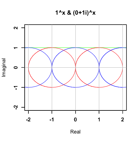
何故周期単位(Cycle Unit)は1でないといけないか、この動きだけで説明出来てしまうんですね。そう、それ以下だと0に収束し、それ以上だと無限に発散して周期を描いてくれないからです。この数理を援用した整数の定義が以下となります。
cx00<-seq(-3,3,length=61)
f0<-function(x) 1^x
cy00<-f0(cx00)
s00<-complex(re=cx00,im=cy00)
plot(s00,type="l",xlim=c(-2,2),ylim=c(-2,2),main="1^x & (0+1i)^x",xlab="Real",ylab="Imaginal",col=rgb(0,1,0))

# -1^x=(0±1i)^2x(i^2=-1)
par(new=T)#上書き
c01<-seq(-1,1,length=61)
f0<-function(x) (0+1i)^x
s01<-f0(cx00)
plot(s01,type="l",xlim=c(-2,2),ylim=c(-2,2),main="",xlab="",ylab="",col=rgb(0,0,1))
par(new=T)#上書き
plot(s01+1,type="l",xlim=c(-2,2),ylim=c(-2,2),main="",xlab="",ylab="",col=rgb(1,0,0))
par(new=T)#上書き
plot(s01-1,type="l",xlim=c(-2,2),ylim=c(-2,2),main="",xlab="",ylab="",col=rgb(1,0,0))
par(new=T)#上書き
plot(s01+2,type="l",xlim=c(-2,2),ylim=c(-2,2),main="",xlab="",ylab="",col=rgb(0,0,1))
par(new=T)#上書き
plot(s01-2,type="l",xlim=c(-2,2),ylim=c(-2,2),main="",xlab="",ylab="",col=rgb(0,0,1))

abline(h=0,col=c(200,200,200))
abline(v=0,col=c(200,200,200))
abline(v=1,col=c(200,200,200))
abline(v=2,col=c(200,200,200))
abline(v=-1,col=c(200,200,200))
abline(v=-2,col=c(200,200,200))
- -1=i^2=(0±1i)^2xすなわち偶数円2nは2n-1→(0+1i)+2n→2n+1→(0-1i)+2n+1→2n,奇数円2n+1は2n→(0+1i)+2n+1→2n+2→(0-1i)+2n+1→2nの4周期を刻む。
- これは偶数円2nが…2n-1→(0+1i)+2n→2n+1→(0-1i)+2n+2→2n+3…奇数円2n+1が…2n→(0+1i)+2n+1→2n+2→(0-1i)+2n+3→2n+4…の周期を無限に刻んでいるととも解釈可能であり、この時離散的に出現する実数y=1^xとの接点が整数集合Zn(N=-Inf→0→Inf){-Inf,…,-1,0,1,…,Inf}となる。
この動きは均等尺を採った円柱座標系上にも、対数尺を採った球面座標系上にも、また大半径1,小半径1のトーラスの連なりとしても表現され得ます。
ところでこの(0±i)^axなる関数、a=0→1の区間では大人しく共役複素数らしい挙動で円弧を描くだけなのですが(実はa=1→2の区間で既に挙動がおかしいので周期単位としては切り捨てを決断)…
【Rで球面幾何学】指数関数や対数関数における「ネイピア数周期」の意味について。 - Qiita
(0+1i)^ax(a=0→1)

Int01<-function(Rad){

cx00<-seq(-3,3,length=61)
f0<-function(x) 1^x
cy00<-f0(cx00)
s00<-complex(re=cx00,im=cy00)
plot(s00,type="l",xlim=c(-2,2),ylim=c(-2,2),main="(0+1i)^ax(a= 0→1)",xlab="Real",ylab="Imaginal",col=rgb(0,1,0))

# -1^x=(0±1i)^2x(i^2=-1)
par(new=T)#上書き
c01<-seq(-1,1,length=61)
f0<-function(x) (0+1i)^(x*Rad)
s01<-f0(cx00)
plot(s01,type="l",xlim=c(-2,2),ylim=c(-2,2),main="",xlab="",ylab="",col=rgb(0,0,1))
par(new=T)#上書き
plot(s01+1,type="l",xlim=c(-2,2),ylim=c(-2,2),main="",xlab="",ylab="",col=rgb(1,0,0))
par(new=T)#上書き
plot(s01-1,type="l",xlim=c(-2,2),ylim=c(-2,2),main="",xlab="",ylab="",col=rgb(1,0,0))
par(new=T)#上書き
plot(s01+2,type="l",xlim=c(-2,2),ylim=c(-2,2),main="",xlab="",ylab="",col=rgb(0,0,1))
par(new=T)#上書き
plot(s01-2,type="l",xlim=c(-2,2),ylim=c(-2,2),main="",xlab="",ylab="",col=rgb(0,0,1))

abline(h=0,col=c(200,200,200))
abline(v=0,col=c(200,200,200))
abline(v=1,col=c(200,200,200))
abline(v=2,col=c(200,200,200))
abline(v=-1,col=c(200,200,200))
abline(v=-2,col=c(200,200,200))

even01<-paste("y=(0+1i)^",Rad,"x(Even)")
odd01<-paste("y=(0+1i)^",Rad,"x(Odd)")

legend("bottomleft", legend=c("y=1^x",even01,odd01), lty =c(1,1,1),col=c(rgb(0,1,0),rgb(0,0,1),rgb(1,0,0)))
}

# アニメーション動作設定
Time_Code<-seq(0,1,length=11)
# アニメーション
library("animation")
saveGIF({
for (i in Time_Code){
 Int01(i)
}
}, interval = 0.1, movie.name = "Int04.gif")
(0-1i)^ax(a=0→1)(共役作用の為、見た目はまるで同じ)

Int01<-function(Rad){

cx00<-seq(-3,3,length=61)
f0<-function(x) 1^x
cy00<-f0(cx00)
s00<-complex(re=cx00,im=cy00)
plot(s00,type="l",xlim=c(-2,2),ylim=c(-2,2),main="(0-1i)^ax(a= 0→1)",xlab="Real",ylab="Imaginal",col=rgb(0,1,0))

# -1^x=(0±1i)^2x(i^2=-1)
par(new=T)#上書き
c01<-seq(-1,1,length=61)
f0<-function(x) (0-1i)^(x*Rad)
s01<-f0(cx00)
plot(s01,type="l",xlim=c(-2,2),ylim=c(-2,2),main="",xlab="",ylab="",col=rgb(0,0,1))
par(new=T)#上書き
plot(s01+1,type="l",xlim=c(-2,2),ylim=c(-2,2),main="",xlab="",ylab="",col=rgb(1,0,0))
par(new=T)#上書き
plot(s01-1,type="l",xlim=c(-2,2),ylim=c(-2,2),main="",xlab="",ylab="",col=rgb(1,0,0))
par(new=T)#上書き
plot(s01+2,type="l",xlim=c(-2,2),ylim=c(-2,2),main="",xlab="",ylab="",col=rgb(0,0,1))
par(new=T)#上書き
plot(s01-2,type="l",xlim=c(-2,2),ylim=c(-2,2),main="",xlab="",ylab="",col=rgb(0,0,1))

abline(h=0,col=c(200,200,200))
abline(v=0,col=c(200,200,200))
abline(v=1,col=c(200,200,200))
abline(v=2,col=c(200,200,200))
abline(v=-1,col=c(200,200,200))
abline(v=-2,col=c(200,200,200))

even01<-paste("y=(0-1i)^",Rad,"x(Even)")
odd01<-paste("y=(0-1i)^",Rad,"x(Odd)")

legend("bottomleft", legend=c("y=1^x",even01,odd01), lty =c(1,1,1),col=c(rgb(0,1,0),rgb(0,0,1),rgb(1,0,0)))
}

# アニメーション動作設定
Time_Code<-seq(0,1,length=11)
# アニメーション
library("animation")
saveGIF({
for (i in Time_Code){
 Int01(i)
}
}, interval = 0.1, movie.name = "Int05.gif")
-(0+1i)^ax(a=0→1)(展開が逆に)

Int01<-function(Rad){

cx00<-seq(-3,3,length=61)
f0<-function(x) 1^x
cy00<-f0(cx00)
s00<-complex(re=cx00,im=cy00)
plot(s00,type="l",xlim=c(-2,2),ylim=c(-2,2),main="-(0+1i)^ax(a= 0→1)",xlab="Real",ylab="Imaginal",col=rgb(0,1,0))

# -1^x=(0±1i)^2x(i^2=-1)
par(new=T)#上書き
c01<-seq(-1,1,length=61)
f0<-function(x) -(0+1i)^(x*Rad)
s01<-f0(cx00)
plot(s01,type="l",xlim=c(-2,2),ylim=c(-2,2),main="",xlab="",ylab="",col=rgb(0,0,1))
par(new=T)#上書き
plot(s01+1,type="l",xlim=c(-2,2),ylim=c(-2,2),main="",xlab="",ylab="",col=rgb(1,0,0))
par(new=T)#上書き
plot(s01-1,type="l",xlim=c(-2,2),ylim=c(-2,2),main="",xlab="",ylab="",col=rgb(1,0,0))
par(new=T)#上書き
plot(s01+2,type="l",xlim=c(-2,2),ylim=c(-2,2),main="",xlab="",ylab="",col=rgb(0,0,1))
par(new=T)#上書き
plot(s01-2,type="l",xlim=c(-2,2),ylim=c(-2,2),main="",xlab="",ylab="",col=rgb(0,0,1))

abline(h=0,col=c(200,200,200))
abline(v=0,col=c(200,200,200))
abline(v=1,col=c(200,200,200))
abline(v=2,col=c(200,200,200))
abline(v=-1,col=c(200,200,200))
abline(v=-2,col=c(200,200,200))

even01<-paste("y=-(0+1i)^",Rad,"x(Even)")
odd01<-paste("y=-(0+1i)^",Rad,"x(Odd)")

legend("bottomleft", legend=c("y=1^x",even01,odd01), lty =c(1,1,1),col=c(rgb(0,1,0),rgb(0,0,1),rgb(1,0,0)))
}

# アニメーション動作設定
Time_Code<-seq(0,1,length=11)
# アニメーション
library("animation")
saveGIF({
for (i in Time_Code){
 Int01(i)
}
}, interval = 0.1, movie.name = "Int06.gif")
aの値がそれ以上になると見た事のない挙動を始めるのです。
(0+1i)^ax(a=0→40)

Int01<-function(Rad,Range){

cx00<-seq(-3,3,length=61)

f0<-function(x) 1^x

cy00<-f0(cx00)

s00<-complex(re=cx00,im=cy00)

title01<-paste("(0+1i)^ax(a=",Range,")")

plot(s00,type="l",xlim=c(-2,2),ylim=c(-2,2),main=title01,xlab="Real",ylab="Imaginal",col=rgb(0,1,0))

# -1^x=(0±1i)^2x(i^2=-1)

par(new=T)#上書き
c01<-seq(-1,1,length=61)
f0<-function(x) (0-1i)^(x*Rad)

s01<-f0(cx00)

plot(s01,type="l",xlim=c(-2,2),ylim=c(-2,2),main="",xlab="",ylab="",col=rgb(0,0,1))

par(new=T)#上書き

plot(s01+1,type="l",xlim=c(-2,2),ylim=c(-2,2),main="",xlab="",ylab="",col=rgb(1,0,0))

par(new=T)#上書き

plot(s01-1,type="l",xlim=c(-2,2),ylim=c(-2,2),main="",xlab="",ylab="",col=rgb(1,0,0))

par(new=T)#上書き

plot(s01+2,type="l",xlim=c(-2,2),ylim=c(-2,2),main="",xlab="",ylab="",col=rgb(0,0,1))

par(new=T)#上書き

plot(s01-2,type="l",xlim=c(-2,2),ylim=c(-2,2),main="",xlab="",ylab="",col=rgb(0,0,1))

abline(h=0,col=c(200,200,200))
abline(v=0,col=c(200,200,200))
abline(v=1,col=c(200,200,200))
abline(v=2,col=c(200,200,200))
abline(v=-1,col=c(200,200,200))
abline(v=-2,col=c(200,200,200))

even01<-paste("y=(0+1i)^",Rad,"x(Even)")
odd01<-paste("y=(0+1i)^",Rad,"x(Odd)")

legend("bottomleft", legend=c("y=1^x",even01,odd01), lty =c(1,1,1),col=c(rgb(0,1,0),rgb(0,0,1),rgb(1,0,0)))

}
# アニメーション動作設定
Time_Code<-seq(0,40,length=201)
# アニメーション
library("animation")
saveGIF({
for (i in Time_Code){
 Int01(i,c("0→40"))
}
}, interval = 0.1, movie.name = "Int11.gif")
(0+1i)^ax(a=0→20)

# アニメーション動作設定
Time_Code<-seq(0,20,length=201)
# アニメーション
library("animation")
saveGIF({
for (i in Time_Code){
 Int01(i,c("0→20"))
}
}, interval = 0.1, movie.name = "Int12.gif")
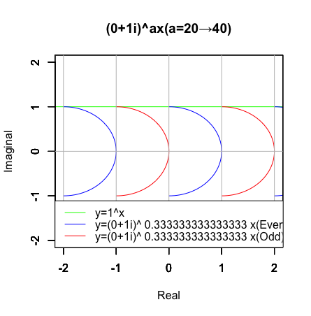
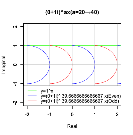
(0+1i)^ax(a=20→40)

# アニメーション動作設定
Time_Code<-seq(20,40,length=201)
# アニメーション
library("animation")
saveGIF({
for (i in Time_Code){
 Int01(i,c("0→20"))
}
}, interval = 0.1, movie.name = "Int13.gif")
要するに傾き次第では周期が「ガウスの巡回群」と一致するのです。
【初心者向け】挟み撃ち定理による円周率πの近似 - Qiita
そしてこれは40進数(40 Base)?英語表現としては20進法(Vigesimal)と60進法(Sexagesimal)しかない様なのでとりあえず倍20進法(Double-Vigesimal)とでも表現するのがもっともらしいかもしれません。
n進法
- a=0から1にかけて(2n+1,0)を起点として共役複素数の作用により中心(2n+1,0)半径1の円が「顕現」。1~20にかけてその円の半径が1→0に推移。
- a=20~39にかけて中心(2n+1,0)の円の半径が0→1に推移。39~40にかけて(2n,0)を終点として共役複素数の作用により中心(2n+1,0)半径1の円が「消失」。
少なくともこの動作はa=-1(39)→0(40)→1の範囲ではθ=-π→0→π、i=0±1iと置き、対数関数(Logarithm Function)log(θi)の底をexp(-1)→exp(0)=1→exp(1)と推移させた場合に対応します。
【Rで球面幾何学】指数関数や対数関数における「ネイピア数周期」の意味について。
-
根に掛ける係数を0(root/root)から1(root)にかけて変化させる->関数X=1を起点に右から左に円弧が「顕現」。

-
根に掛ける係数を-1(1/root)から0(root/root)にかけて変化させる->関数X=1を起点に左から右に円弧が「消失」。

-
-log(θi)では関数X=-1を起点に逆展開。


指数関数(Exponential Function)e^θiの底をexp(-1)→exp(0)=1→exp(1)と推移させるとこれに直交する結果が得られます。
-
根に掛ける係数を0(root/root)から1(root)にかけて変化させる->関数Y=1を起点に上から下に円弧が「顕現」。

-
根に掛ける係数を-1(1/root)から0(root/root)にかけて変化させる->関数Y=1を起点に下から上に円弧が「消失」。

-
-log(θi)では関数Y=-1を起点に逆展開。


こうした全体像を俯瞰したのが以下の「共役球面(Conjugated Sphere)」となる訳です。あえて定義するなら「その球面上の任意の対蹠(Antipodes)間を結ぶ距離空間(Distance Space)」といったところですか。
【初心者向け】複素共役のアニメーション表示について。


-
球面座標管理や球面描画はこの考え方から出発するが、それだけだとジンバルロック(Gimbal lock)問題を回避出来ない。
[【初心者向け】「単位円筒」から「単位球面」へ]
(https://qiita.com/ochimusha01/items/08f5c5ad1aba4a59a27d)
- 一方、この座標系(Coordinate System)はオイラーの公式e^θi/log(θi)の応用によりφ(-π→0→π)、θ(-π→0→π)の2軸の平面極座標(Plane Polar Coordinates System)によっても任意の点の位置を表せる。自明の場合としてジンバルロック問題は生じない。四元数(Quaternion)の正規部分解表現(Sympletic Form)に該当。
Rの四元数ライブラリOnion
【Rで球面幾何学】ジンバルロック(?)やリサージュ曲線(?)との邂逅。
それはともかく(2n,0)を起点とする共役複素数の作用によりa=1/3(39+2/3=39.66667)の時半円が…
…a=1/6(39+5/6=39.83333)の時四分円が「顕現」する訳ですが…
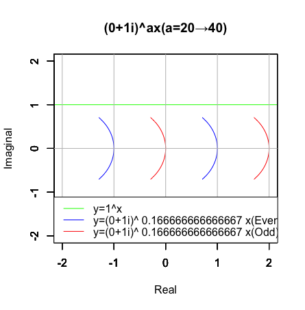
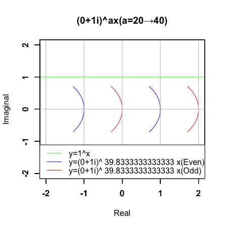
半円が整数直線(Integer Line)y=1^xに1/2(0.5)の位置で接するのに対し、変化の範囲を1未満に限るとそれ以上でもそれ以下でも接しません。なるほどこれが2進法(Binary)に立脚する偶奇性(Parity)概念の大源流となる訳ですね。三角不等式‖x+y‖≦‖x‖+‖y‖の適用範囲が原則として‖x+y‖=‖x‖+‖y‖のみととなる整数直線の世界をさらに二分する概念(Concept)の導入(Introduce)という訳です。しかもそこには既に素数3^n族の影が…
この数理(Mathematical Thing)についてまだまだ色々と調べないといけません。そんな感じで以下続報…