前回の記事に続き、今度はメインである可視化処理を読み込んでいきます。
可視化
まずは可視化のコード「test.caltech.py」を読み込んでいきます。
インポートライブラリ
今回の処理で必要になるライブラリは以下の通りです。
import tensorflow as tf
import pandas as pd
import numpy as np

from detector import Detector
from util import load_image

import skimage.io
import matplotlib.pyplot as plt

import os
import ipdb
前回から「Matplotlib」が増えています。
呼び出すファイルの方は、前回と同じなので省略します。
※結局Anacondaで環境作って、TensorFlowを追加すれば大丈夫そう
入出力パス/ファイル
基本的な構造はトレーニング(train.caltech.py)と同じなので、ここでの説明も同じように進めていきます。
インポートの次には、入出力に関連するパス名やファイル名の指定があります。
testset_path = '../data/caltech/test.pickle'
label_dict_path = '../data/caltech/label_dict.pickle'

weight_path = '../data/caffe_layers_value.pickle'
model_path = '../models/caltech256/model-4'
これらのファイルはトレーニング時にできているはずです。
「model_path」は、使用したい学習済みモデルを指定します。
※「model-4」はepochを4回回した結果です
定数定義
次に定数を定義しています。
batch_size = 1
可視化処理では1枚づつ画像を処理していきます。
データリストの作成
可視化の入力となる画像ファイルのリスト(トレーニング時にはテストで使用)とラベルのリストを用意します。
testset = pd.read_pickle( testset_path )[::-1][:20]
label_dict = pd.read_pickle( label_dict_path )
n_labels = len( label_dict )
推論(Inference)
続いて、「推論(Inference)」の処理を定義していきます。
images_tf = tf.placeholder( tf.float32, [None, 224, 224, 3], name="images")
labels_tf = tf.placeholder( tf.int64, [None], name='labels')
detector = Detector( weight_path, n_labels )
c1,c2,c3,c4,conv5, conv6, gap, output = detector.inference( images_tf )
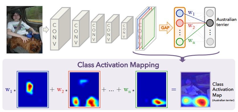
classmap = detector.get_classmap( labels_tf, conv6 )
最後の1行だけ、トレーニング時と異なります。
ここでは畳み込み処理の最後の状態から、クラスマップ(後述)を取得します。
実際の処理は、別のファイル(detector.py)で行っています。
    def get_classmap(self, label, conv6):
        conv6_resized = tf.image.resize_bilinear( conv6, [224, 224] )
        with tf.variable_scope("GAP", reuse=True):
            label_w = tf.gather(tf.transpose(tf.get_variable("W")), label)
            label_w = tf.reshape( label_w, [-1, 1024, 1] ) # [batch_size, 1024, 1]

        conv6_resized = tf.reshape(conv6_resized, [-1, 224*224, 1024]) # [batch_size, 224*224, 1024]

        classmap = tf.batch_matmul( conv6_resized, label_w )
        classmap = tf.reshape( classmap, [-1, 224,224] )
        return classmap
まず、縦14x横14x1024チャンネルの画像を縦224x横224x1024チャンネルに拡大します。
その後、トレーニング時に作成したGAPのweightを取得し、転置してから、指定したラベルへの重みだけ取り出して1024x1に変換します。
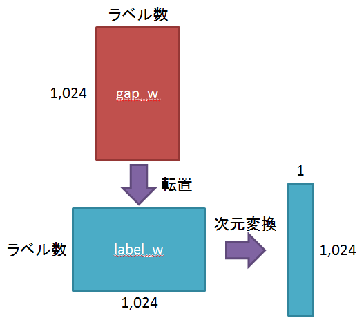
さらに、拡大した画像を縦224*224x横1024の1枚の画像に変換し、前述の1024x1のweightと掛け合わせ、クラスマップを生成します。
最後に縦244x横244の画像に変換します。
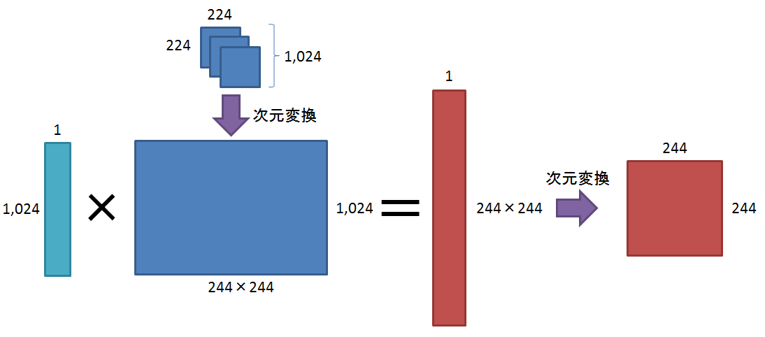
なお、この時点では画像はグレースケールになります。
(最後の表示時に色づけしています)
処理の実行
初期化
まずはセッションを用意します。
sess = tf.InteractiveSession()
saver = tf.train.Saver()
学習済モデルの読み込み
トレーニングで作成した学習済みモデルを読み込みます。
saver.restore( sess, model_path )
バッチ単位の処理
ここからバッチサイズごとの処理を行います。
なお、今回はバッチサイズが1ですので、実際には画像を1枚づつ処理することになります。
for start, end in zip(
    range( 0, len(testset)+batch_size, batch_size),
    range(batch_size, len(testset)+batch_size, batch_size)):

    current_data = testset[start:end]
    current_image_paths = current_data['image_path'].values
    current_images = np.array(map(lambda x: load_image(x), current_image_paths))

    good_index = np.array(map(lambda x: x is not None, current_images))

    current_data = current_data[good_index]
    current_image_paths = current_image_paths[good_index]
    current_images = np.stack(current_images[good_index])
    current_labels = current_data['label'].values
    current_label_names = current_data['label_name'].values

    conv6_val, output_val = sess.run(
            [conv6, output],
            feed_dict={
                images_tf: current_images
                })
まずバッチ数分の画像を読み込みます。
一応念のため、ファイルがあったかのフラグを用意します。
存在したものだけを処理するため、改めて画像とラベルのリストを作成します。
その後、トレーニングを実行します。
ここでの出力は、畳み込み処理を行った後の状態になります。
※クラスマップではありません
バッチ単位の処理(つづき)
この後の処理がメインになります。
    label_predictions = output_val.argmax( axis=1 )
    acc = (label_predictions == current_labels).sum()

    classmap_vals = sess.run(
            classmap,
            feed_dict={
                labels_tf: label_predictions,
                conv6: conv6_val
                })

    classmap_answer = sess.run(
            classmap,
            feed_dict={
                labels_tf: current_labels,
                conv6: conv6_val
                })

    classmap_vis = map(lambda x: ((x-x.min())/(x.max()-x.min())), classmap_answer)

    for vis, ori,ori_path, l_name in zip(classmap_vis, current_images, current_image_paths, current_label_names):
        print l_name
        plt.imshow( ori )
        plt.imshow( vis, cmap=plt.cm.jet, alpha=0.5, interpolation='nearest' )
        plt.show()
識別結果の一番大きい値から、何であると判断されたかを取得します。
その後、識別されたラベルでのクラスマップと、正解ラベルのクラスマップを作成します。
正解ラベルのクラスマップを0~1に正規化し、画像を表示します。(バッチ数が1なので、1枚だけ表示されます)
なお、識別されたラベルのクラスマップは使用されません。
このソースでは、「正解は○○で、ここを注目したため、正解/不正解でした」という可視化になっているようです。
識別された方を使えば、「ここを注目してしまったため、正解/不正解となりました」という可視化ができると思います。
画像の保存
一番最後に、作成した画像を保存します。
ただ、現在はコメントアウトされています。
#        vis_path = '../results/'+ ori_path.split('/')[-1]
#        vis_path_ori = '../results/'+ori_path.split('/')[-1].split('.')[0]+'.ori.jpg'
#        skimage.io.imsave( vis_path, vis )
#        skimage.io.imsave( vis_path_ori, ori )
まとめ
クラスマップの作成部分がメインなのですが、分かりづらく、なかなかつらかったです。
今後はオリジナルの学習データを使用して、CAMを試してみたいと思います。
また、後継のGrad-CAMもお勉強してみたいと考えています。