Class Activation Mapping（CAM）の実装である「Weakly_detector」のソースを読み解く ～トレーニング編～

Deep Learningのお仕事をしていると、お客様から「なんでこういう結果になるの？」という質問をよく頂きます。

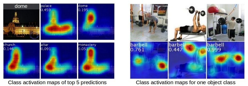
その際利用するのが「注目位置の可視化」なのですが、その一つの例である「Class Activation Mapping（CAM）」の処理を理解するために、実装コードである「Weakly_detector」を読み込んでみます。

ちなみに、「Weakly_detector」のソースコードはGitHubで公開されています。

トレーニング

まずはトレーニングのコード「train.caltech.py」を読み込んでいきます。

インポートライブラリ

今回の処理で必要になるライブラリは以下の通りです。

train.caltech.py

import tensorflow as tf
import numpy as np
import pandas as pd

from detector import Detector
from util import load_image
import os
import ipdb

また、呼び出している関数が定義されている別のファイル（detector.py、util.py）でも、他のライブラリを利用しています。

detector.py

import tensorflow as tf
import numpy as np
import cPickle
import ipdb

util.py

import skimage.io
import skimage.transform
import ipdb

import numpy as np

よって、外部モジュールとして「TensorFlow」「NumPy」「pandas」「scikit-image」が必要になります。

※結局Anacondaで環境作って、TensorFlowを追加すれば大丈夫そう

入出力パス／ファイル

次に、入出力に関連するパス名やファイル名の指定があります。

weight_path = '../data/caffe_layers_value.pickle'
model_path = '../models/caltech256/'
pretrained_model_path = None #'../models/caltech256/model-0'

dataset_path = '/media/storage3/Study/data/256_ObjectCategories'

caltech_path = '../data/caltech'
trainset_path = '../data/caltech/train.pickle'
testset_path = '../data/caltech/test.pickle'
label_dict_path = '../data/caltech/label_dict.pickle'

必ず事前に準備が必要なのは、「dataset_path」で指定されている学習データセットになります。
今回はCaltech-256を使用しています。こちらからダウンロードしておきます。
学習データは、それぞれ「nnn.label_name」（nnnは001～257までの数字、label_nameはラベル名）の形式で命名されたディレクトリ内に保存されています。
学習データ自体は、「nnn_mmmm.jpg」（nnnは001～257までの数字、mmmmは0001～の数字）になっています。

ちなみに、今回使用する学習データは、サイズも縦横比もバラバラです。
そのため全ての学習データが同じサイズになるように、読み込んだ後正方形に切り出してからリサイズしています。

また「weight_path」も必要になりますが、これはGitHubのところから辿れるリンク先から取得してください。
この中で設定されている、畳み込みレイヤーのweightやbiasを利用しています。（ファインチューニング）

他はトレーニングでできるファイル等です。
もしすでにトレーニング済みであれば、これらのパスにファイルが存在しているはずですので、そこに続けてトレーニングを行うことになります。

定数定義

前述の入出力パスと同時に、いくつかの定数を定義しています。

n_epochs = 10000
init_learning_rate = 0.01
weight_decay_rate = 0.0005
momentum = 0.9
batch_size = 60

これらは学習時のパラメータとして使用されます。
もちろん変更することで調整が可能です。

学習データリストの作成

ここから、ようやくトレーニングに向けた処理が始まります。

まず初めにトレーニング、および、テストで使用する学習データのリストを作成します。

if not os.path.exists( trainset_path ):
    if not os.path.exists( caltech_path ):
        os.makedirs( caltech_path )
    image_dir_list = os.listdir( dataset_path )

    label_pairs = map(lambda x: x.split('.'), image_dir_list)
    labels, label_names = zip(*label_pairs)
    labels = map(lambda x: int(x), labels)

    label_dict = pd.Series( labels, index=label_names )
    label_dict -= 1
    n_labels = len( label_dict )

    image_paths_per_label = map(lambda one_dir: map(lambda one_file: os.path.join( dataset_path, one_dir, one_file ), os.listdir( os.path.join( dataset_path, one_dir))), image_dir_list)
    image_paths_train = np.hstack(map(lambda one_class: one_class[:-10], image_paths_per_label))
    image_paths_test = np.hstack(map(lambda one_class: one_class[-10:], image_paths_per_label))

    trainset = pd.DataFrame({'image_path': image_paths_train})
    testset  = pd.DataFrame({'image_path': image_paths_test })

    trainset = trainset[ trainset['image_path'].map( lambda x: x.endswith('.jpg'))]
    trainset['label'] = trainset['image_path'].map(lambda x: int(x.split('/')[-2].split('.')[0]) - 1)
    trainset['label_name'] = trainset['image_path'].map(lambda x: x.split('/')[-2].split('.')[1])

    testset = testset[ testset['image_path'].map( lambda x: x.endswith('.jpg'))]
    testset['label'] = testset['image_path'].map(lambda x: int(x.split('/')[-2].split('.')[0]) - 1)
    testset['label_name'] = testset['image_path'].map(lambda x: x.split('/')[-2].split('.')[1])

    label_dict.to_pickle(label_dict_path)
    trainset.to_pickle(trainset_path)
    testset.to_pickle(testset_path)
else:
    trainset = pd.read_pickle( trainset_path )
    testset  = pd.read_pickle( testset_path )
    label_dict = pd.read_pickle( label_dict_path )
    n_labels = len(label_dict)

まず学習データセットの各ディレクトリ名がlabel_pairsに保存されます。
それをラベルとラベル名に分割して、labels・label_namesに保存します。（labelsは文字列から数値に変換します）
ラベル名を1次元配列label_dictに格納し、ラベル数をn_labelsに設定しておきます。

それぞれのラベルにおいて、その中に設定されている学習データの内10個をテスト用とし、残りをトレーニング用とします。
これらはNumPyのDataFrameの形式で保存され、各レコードは「image_path（画像ファイル名）」「label（ラベル）」「label_name（ラベル名）」で構成されます。

出来上がったDaraFrameはPicklingしてファイル化しています。
作成済みの場合は、Picklingしたファイルを読み込んでいます。

【余談】Pickling

Python初心者の私には、「Pickling」が何のことかわかりませんでした（苦笑）
・・・ピクルスとは関係ないことは、うすうす気づいていましたが ^^;
いわゆる「シリアライズ」のようです。
詳しくはこの辺りを参考にしてみてください。

これらの処理は、Pandasの関数として実装されており、今回はそれをそのまま使用しています。

推論（Inference）

ここからはTensorFlowでの実装パターンでいうところの「推論（Inference）」の処理になります。

learning_rate = tf.placeholder( tf.float32, [])
images_tf = tf.placeholder( tf.float32, [None, 224, 224, 3], name="images")
labels_tf = tf.placeholder( tf.int64, [None], name='labels')

detector = Detector(weight_path, n_labels)

p1,p2,p3,p4,conv5, conv6, gap, output = detector.inference(images_tf)

まず受け渡しの変数であるplaceholder（入力画像用、出力ラベル用）を用意します。さらに、ここでは学習レートも変数として用意しています。
なお、今回の学習データは224x224で3チャンネル（RGB）の画像になります。

次にネットワークモデルを定義しています。
「Detector()」の中身は別のファイルで定義されています。

detector.py

import tensorflow as tf
import numpy as np
import cPickle
import ipdb
class Detector():
    def __init__(self, weight_file_path, n_labels):
        self.image_mean = [103.939, 116.779, 123.68]
        self.n_labels = n_labels

        with open(weight_file_path) as f:
            self.pretrained_weights = cPickle.load(f)

    def get_weight( self, layer_name):
        layer = self.pretrained_weights[layer_name]
        return layer[0]

    def get_bias( self, layer_name ):
        layer = self.pretrained_weights[layer_name]
        return layer[1]

    def get_conv_weight( self, name ):
        f = self.get_weight( name )
        return f.transpose(( 2,3,1,0 ))

    def conv_layer( self, bottom, name ):
        with tf.variable_scope(name) as scope:

            w = self.get_conv_weight(name)
            b = self.get_bias(name)

            conv_weights = tf.get_variable(
                    "W",
                    shape=w.shape,
                    initializer=tf.constant_initializer(w)
                    )
            conv_biases = tf.get_variable(
                    "b",
                    shape=b.shape,
                    initializer=tf.constant_initializer(b)
                    )

            conv = tf.nn.conv2d( bottom, conv_weights, [1,1,1,1], padding='SAME')
            bias = tf.nn.bias_add( conv, conv_biases )
            relu = tf.nn.relu( bias, name=name )

        return relu

    def new_conv_layer( self, bottom, filter_shape, name ):
        with tf.variable_scope( name ) as scope:
            w = tf.get_variable(
                    "W",
                    shape=filter_shape,
                    initializer=tf.random_normal_initializer(0., 0.01))
            b = tf.get_variable(
                    "b",
                    shape=filter_shape[-1],
                    initializer=tf.constant_initializer(0.))

            conv = tf.nn.conv2d( bottom, w, [1,1,1,1], padding='SAME')
            bias = tf.nn.bias_add(conv, b)

        return bias #relu

    def inference( self, rgb, train=False ):
        rgb *= 255.
        r, g, b = tf.split(3, 3, rgb)
        bgr = tf.concat(3,
            [
                b-self.image_mean[0],
                g-self.image_mean[1],
                r-self.image_mean[2]
            ])

        relu1_1 = self.conv_layer( bgr, "conv1_1" )
        relu1_2 = self.conv_layer( relu1_1, "conv1_2" )

        pool1 = tf.nn.max_pool(relu1_2, ksize=[1, 2, 2, 1], strides=[1, 2, 2, 1],
                                         padding='SAME', name='pool1')

        relu2_1 = self.conv_layer(pool1, "conv2_1")
        relu2_2 = self.conv_layer(relu2_1, "conv2_2")
        pool2 = tf.nn.max_pool(relu2_2, ksize=[1, 2, 2, 1], strides=[1, 2, 2, 1],
                               padding='SAME', name='pool2')

        relu3_1 = self.conv_layer( pool2, "conv3_1")
        relu3_2 = self.conv_layer( relu3_1, "conv3_2")
        relu3_3 = self.conv_layer( relu3_2, "conv3_3")
        pool3 = tf.nn.max_pool(relu3_3, ksize=[1, 2, 2, 1], strides=[1, 2, 2, 1],
                               padding='SAME', name='pool3')

        relu4_1 = self.conv_layer( pool3, "conv4_1")
        relu4_2 = self.conv_layer( relu4_1, "conv4_2")
        relu4_3 = self.conv_layer( relu4_2, "conv4_3")
        pool4 = tf.nn.max_pool(relu4_3, ksize=[1, 2, 2, 1], strides=[1, 2, 2, 1],
                               padding='SAME', name='pool4')

        relu5_1 = self.conv_layer( pool4, "conv5_1")
        relu5_2 = self.conv_layer( relu5_1, "conv5_2")
        relu5_3 = self.conv_layer( relu5_2, "conv5_3")

        conv6 = self.new_conv_layer( relu5_3, [3,3,512,1024], "conv6")
        gap = tf.reduce_mean( conv6, [1,2] )

        with tf.variable_scope("GAP"):
            gap_w = tf.get_variable(
                    "W",
                    shape=[1024, self.n_labels],
                    initializer=tf.random_normal_initializer(0., 0.01))

        output = tf.matmul( gap, gap_w)

        return pool1, pool2, pool3, pool4, relu5_3, conv6, gap, output

いきなり255倍していてガックリしますが（笑）、RGBの画像をBGRの3プレーンに変換します。その際、平均画素値（平均画像ではなく、しかも決め打ちｗｗｗ）を引いて平均化しています。
その後、
・conv→conv→max pool（224x224→112x112）
・conv→conv→max pool（112x112→56x56）
・conv→conv→conv→max pool（56x56→28x28）
・conv→conv→conv→max pool（28x28→14x14）
・conv→conv→conv
・conv*（ReLU無し）
と処理を重ね、最後に全結合（1024→レベル数）を行います。

※このモデルの元は「VGGnet」になります

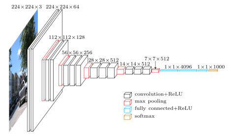
　最後のmax pooling以降を取り除き、conv*とGAP+Softmaxを追加した構造になっています
　ちなみに元の論文では「AlexNet」や「GoogLeNet」でも評価しています

convで使用するweightやbiasは、読み込んだ「weight_path」に設定されている値を使用する（ファインチューニング）ため、このソースからは分かりません．．．
※strideは1画素づつ移動
またconvでは活性化関数としてReLUを使用します。

max poolでは2x2でプーリングを行い、strideも2画素づつとなっています。
（画像サイズが半分になります）

最後のconv*では、フィルターのサイズが縦3x横3で、512チャンネルを1024チャンネルに拡張するように畳み込みを行います。
また、ここではプーリングは行いません。
ちなみに、このconv*の結果（縦14x横14x1024チャンネル）を、CAMの可視化処理で使用します。

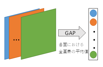
その後、チャンネル毎に平均を計算します。
（この時点で要素1024個の1次元配列にします）
この処理に事を「Global Average Pooling（GAP）」と呼びます。

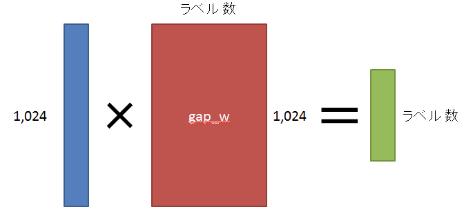
最後に、最終的にレベル数になるように全結合計算を行います。

目標値との誤差（Loss）

次に目標値との誤差（Loss）を指定します。

loss_tf = tf.reduce_mean(tf.nn.sparse_softmax_cross_entropy_with_logits( output, labels_tf ))

ここではSoftmax関数（交差エントロピー）を使用しています。

最適化のアルゴリズム（Training）

最後に最適化のアルゴリズム（Training）を指定します。

weights_only = filter( lambda x: x.name.endswith('W:0'), tf.trainable_variables() )
weight_decay = tf.reduce_sum(tf.pack([tf.nn.l2_loss(x) for x in weights_only])) * weight_decay_rate
loss_tf += weight_decay

さらに、オプティマイザの設定も行っています。

optimizer = tf.train.MomentumOptimizer( learning_rate, momentum )
grads_and_vars = optimizer.compute_gradients( loss_tf )
grads_and_vars = map(lambda gv: (gv[0], gv[1]) if ('conv6' in gv[1].name or 'GAP' in gv[1].name) else (gv[0]*0.1, gv[1]), grads_and_vars)
#grads_and_vars = [(tf.clip_by_value(gv[0], -5., 5.), gv[1]) for gv in grads_and_vars]
train_op = optimizer.apply_gradients( grads_and_vars )

なお、オプティマイザに関しては勉強不足で、その効果や意味などは理解できていません。
もっとお勉強します．．．

処理の実行

初期化

まずはセッションを用意します。

sess = tf.InteractiveSession()
saver = tf.train.Saver( max_to_keep=50 )

saverは、epoch単位で学習済みモデルを出力するために用意しています。
この後にオプティマイザの設定を行い、続けて初期化を行っています。

tf.initialize_all_variables().run()

学習済モデルの読み込み

もし学習済みモデルがあるのであれば、ここで読み込み、継続して更新して行きます。

if pretrained_model_path:
    print "Pretrained"
    saver.restore(sess, pretrained_model_path)

インデックスの設定

ここでテスト用データにインデックスを設定しています。
インデックスの設定はもっと後でもかまわないのですが、コメント部分の処理の都合や見やすさから、ここにあるようです。

※トレーニング用のデータはepochごとに並べ替えていますが、テスト用のデータは並び替える必要がないため、ループの外にあるようです

testset.index  = range( len(testset) )
#testset = testset.ix[np.random.permutation( len(testset) )]#[:1000]
#trainset2 = testset[1000:]
#testset = testset[:1000]

#trainset = pd.concat( [trainset, trainset2] )
# We lack the number of training set. Let's use some of the test images

コメント部分は、テスト用データの一部をトレーニング用に追加する処理になります。
トレーニング用の学習データが足らない時に、この処理を有効にするとかする感じかと思います。

【余談】#とか[]とか:とか

Python初心者には、何を表しているのかよくわからないです（涙）
C/C++の知識が邪魔になります．．．

ログ出力の準備

ログ出力するファイルを用意しています。

f_log = open('../results/log.caltech256.txt', 'w')

epoch単位の処理

ここからepoch単位に処理を行っていきます。

iterations = 0
loss_list = []
for epoch in range(n_epochs):

    trainset.index = range( len(trainset) )
    trainset = trainset.ix[ np.random.permutation( len(trainset) )]

    for start, end in zip(
        range( 0, len(trainset)+batch_size, batch_size),
        range(batch_size, len(trainset)+batch_size, batch_size)):

        current_data = trainset[start:end]
        current_image_paths = current_data['image_path'].values
        current_images = np.array(map(lambda x: load_image(x), current_image_paths))

        good_index = np.array(map(lambda x: x is not None, current_images))

        current_data = current_data[good_index]
        current_images = np.stack(current_images[good_index])
        current_labels = current_data['label'].values

        _, loss_val, output_val = sess.run(
                [train_op, loss_tf, output],
                feed_dict={
                    learning_rate: init_learning_rate,
                    images_tf: current_images,
                    labels_tf: current_labels
                    })

        loss_list.append( loss_val )

        iterations += 1
        if iterations % 5 == 0:
            print "======================================"
            print "Epoch", epoch, "Iteration", iterations
            print "Processed", start, '/', len(trainset)

            label_predictions = output_val.argmax(axis=1)
            acc = (label_predictions == current_labels).sum()

            print "Accuracy:", acc, '/', len(current_labels)
            print "Training Loss:", np.mean(loss_list)
            print "\n"
            loss_list = []

    n_correct = 0
    n_data = 0
    for start, end in zip(
            range(0, len(testset)+batch_size, batch_size),
            range(batch_size, len(testset)+batch_size, batch_size)
            ):
        current_data = testset[start:end]
        current_image_paths = current_data['image_path'].values
        current_images = np.array(map(lambda x: load_image(x), current_image_paths))

        good_index = np.array(map(lambda x: x is not None, current_images))

        current_data = current_data[good_index]
        current_images = np.stack(current_images[good_index])
        current_labels = current_data['label'].values

        output_vals = sess.run(
                output,
                feed_dict={images_tf:current_images})

        label_predictions = output_vals.argmax(axis=1)
        acc = (label_predictions == current_labels).sum()

        n_correct += acc
        n_data += len(current_data)

    acc_all = n_correct / float(n_data)
    f_log.write('epoch:'+str(epoch)+'\tacc:'+str(acc_all) + '\n')
    print "$$$$$$$$$$$$$$$$$$$$$$$$$$$$$$$$$$$$$$$$$$$$$$$"
    print 'epoch:'+str(epoch)+'\tacc:'+str(acc_all) + '\n'
    print "$$$$$$$$$$$$$$$$$$$$$$$$$$$$$$$$$$$$$$$$$$$$$$$"

    saver.save( sess, os.path.join( model_path, 'model'), global_step=epoch)

    init_learning_rate *= 0.99

まず、ごっそりトレーニング用データを取得し、ランダムに並べ替えます。
※よって、epoch単位に学習のたびに結果が変わってきます

次にミニバッチのサイズでぐりぐり回していきます。
なお、このミニバッチのループは2つあり、つまり2つの出力（実行処理）を行います。
1つ目がトレーニングのためのループで、1つ目がテストのためのループになります。
トレーニング経過は、1つ目のループで出力しています。

【余談】zip

ループで使うと便利とのうわさの「zip」。当然知りませんでした（爆）
同時に複数の変数で回していくときに使えるようです。
ループ数は、数の少ない方になるようです。

epoch単位の処理（つづき）

まずバッチ数分の画像を読み込みます。
実際に画像ファイルを読み込んでいるのは「load_image()」になります。
こちらは別ファイルで定義されています。

util.py

import skimage.io
import skimage.transform
import ipdb

import numpy as np

def load_image( path ):
    try:
        img = skimage.io.imread( path ).astype( float )
    except:
        return None

    if img is None: return None
    if len(img.shape) < 2: return None
    if len(img.shape) == 4: return None
    if len(img.shape) == 2: img=np.tile(img[:,:,None], 3)
    if img.shape[2] == 4: img=img[:,:,:3]
    if img.shape[2] > 4: return None

    img /= 255.

    short_edge = min( img.shape[:2] )
    yy = int((img.shape[0] - short_edge) / 2)
    xx = int((img.shape[1] - short_edge) / 2)
    crop_img = img[yy:yy+short_edge, xx:xx+short_edge]
    resized_img = skimage.transform.resize( crop_img, [224,224] )
    return resized_img

画像ファイルの読み込みはscikit-imageを使用しています。
読み込み後、各画素の値を0～1に正規化し、さらに一旦正方形にクロップしてから画像サイズを224x224にリサイズしています。

画像ファイル読み込み処理後、一応念のため、ファイルがあったかのフラグを用意します。
存在したものだけを処理するため、改めて画像とラベルのリストを作成します。

その後、トレーニングを実行します。
（2つ目のループではテストを実行）

epoch分の処理が終わるとテスト結果を表示し、学習済みモデルを作成（ファイル出力）します。
このファイルは、識別処理時に使用します。

まとめ

とりあえずトレーニングに関しては、通常と大きく異なる処理は行っていません。
重要なところは、識別処理の方になります。

※続きはこちら