influence functionとは

ICML2017のベストペーパーであるUnderstanding Black-box Predictions via Influence Functionsで提案された関数で，機械学習モデルに対して学習サンプルが与える摂動を定式化したものです．

論文の概要や解説についてはこちらやこちらをご参照ください．

この記事では，influence functionの挙動を理解するためにいくつかの実験をします．

ロジスティック回帰とinfluence function

ロジスティック回帰はこちらの実装を参考にさせていただきます．

irisデータセットを使用します

import numpy as np
import matplotlib.pyplot as plt
from sklearn.preprocessing import StandardScaler
from sklearn.datasets import load_iris

# irisデータセット
iris = load_iris()

# setosaとversicolorの萼片の長さ・幅のみを使う
X = iris.data[iris.target != 2][:, :2]
Y = iris.target[iris.target != 2]

# 標準化
X = StandardScaler().fit_transform(X)

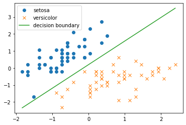
# 散布図
plt.scatter(X[:,0][Y == 0], X[:,1][Y == 0], label=iris.target_names[0], marker='o') 
plt.scatter(X[:,0][Y == 1], X[:,1][Y == 1], label=iris.target_names[1], marker='x')
plt.legend()
plt.show()

まずは普通にロジスティック回帰を実装して，irisデータセットに適用し，決定境界を図示します．

def sigmoid(x):
    """シグモイド関数"""
    return 1 / (1 + np.exp(-x))

def logistic_regression(X,Y):
    """ロジスティック回帰"""
    ETA = 1e-3  # 学習率
    epochs = 5000  # 更新回数

    # バイアス項の計算のために０列目を追加
    X = np.hstack([np.ones([X.shape[0],1]),X])

    # パラメータの初期化
    theta = np.random.rand(3)

    print('更新前のパラメータθ')
    print(theta)

    # パラメータの更新
    for _ in range(epochs):
        theta = theta + ETA * np.dot(Y - sigmoid(np.dot(X, theta)), X)

    print('更新後のパラメータθ')
    print(theta)

    print('決定境界')
    print('y = {:0.3f} + {:0.3f} * x1 + {:0.3f} * x2'.format(theta[0], theta[1], theta[2]))

    return theta

def decision_boundary(xline, theta):
    """決定境界"""
    return -(theta[0] + theta[1] * xline) / theta[2]

theta = logistic_regression(X,Y)

#標本データのプロット
plt.plot(X[Y==0, 0],X[Y==0,1],'o', label=iris.target_names[0])
plt.plot(X[Y==1, 0],X[Y==1,1],'x', label=iris.target_names[1])

xline = np.linspace(np.min(X[:,0]),np.max(X[:,0]),100)

# 決定境界のプロット
plt.plot(xline, decision_boundary(xline, theta), label='decision boundary')
plt.legend()
plt.show()

次に，influence関数を実装します．（実装が間違っていたらすみません！）

# influence関数はy in {1,-1} として計算するので，Yをそのように変換
Y1 = np.copy(Y)
Y1[Y1==0] = -1

# バイアス項の計算のために０列目を追加
X1 = np.hstack([np.ones([X.shape[0],1]),X])

def get_influence(x,y,theta):
    """influence関数"""
    H = (1/X1.shape[0]) * np.sum(np.array([sigmoid(np.dot(xi, theta)) * sigmoid(-np.dot(xi, theta)) * np.dot(xi.reshape(-1,1), xi.reshape(1,-1)) for xi in X1]), axis=0)
    return - y * sigmoid(- y * np.dot(theta, x)) * np.dot(-Y1 * sigmoid(np.dot(Y1, np.dot(theta, X1.T))), np.dot(x, np.dot(np.linalg.inv(H), X1.T)))

# 各サンプルのinfluence値からなるリスト
influence_list = [get_influence(x,y,theta) for x,y in zip(X1,Y1)]

# influence値も含めてプロット
plt.figure(figsize=(12,8))
plt.plot(X[Y==0, 0],X[Y==0,1],'o')
plt.plot(X[Y==1, 0],X[Y==1,1],'x')
plt.plot(xline, decision_boundary(xline, theta), label='decision boundary')
# influence値をグラフに挿入
for x,influence in zip(X, influence_list):
    plt.annotate(f"{influence:.1f}", xy=(x[0], x[1]), size=10)
plt.legend()
plt.show()

個々のサンプルのinfluence値を一緒にプロットすると下図のようになります．

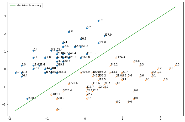
決定境界に近いサンプルほどinfluence値が高いことがわかります．

ミスラベルを意図的に混入させた場合

ミスラベルとは，誤ったラベルのことで，これがあるとモデルが間違った学習をしたり，適切な評価ができなくなったりします．

ここでは，意図的なミスラベルを混入させて，influence値がどのようになるか調べます．

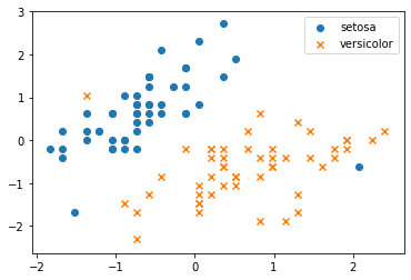
一部のラベルを意図的に付け替えます．下図を見ると，明らかに間違ったラベルがあることがわかると思います．

# 一部のラベルを意図的に入れ替える
Y[76] = 0
Y[22] = 1

# 散布図
plt.scatter(X[:,0][Y == 0], X[:,1][Y == 0], label=iris.target_names[0], marker='o') 
plt.scatter(X[:,0][Y == 1], X[:,1][Y == 1], label=iris.target_names[1], marker='x')
plt.legend()
plt.show()

このデータに対して，上と同じようにロジスティック回帰を適用して，さらにinfluence値を計算して図示すると，以下のようになります．

theta = logistic_regression(X,Y)

# influence関数はy in {1,-1} として計算するので，Yをそのように変換
Y1 = np.copy(Y)
Y1[Y1==0] = -1

# バイアス項の計算のために０列目を追加
X1 = np.hstack([np.ones([X.shape[0],1]),X])

def get_influence(x,y,theta):
    """influence関数"""
    H = (1/X1.shape[0]) * np.sum(np.array([sigmoid(np.dot(xi, theta)) * sigmoid(-np.dot(xi, theta)) * np.dot(xi.reshape(-1,1), xi.reshape(1,-1)) for xi in X1]), axis=0)
    return - y * sigmoid(- y * np.dot(theta, x)) * np.dot(-Y1 * sigmoid(np.dot(Y1, np.dot(theta, X1.T))), np.dot(x, np.dot(np.linalg.inv(H), X1.T)))

# 各サンプルのinfluence値からなるリスト
influence_list = [get_influence(x,y,theta) for x,y in zip(X1,Y1)]

# influence値も含めてプロット
plt.figure(figsize=(12,8))
plt.plot(X[Y==0, 0],X[Y==0,1],'o')
plt.plot(X[Y==1, 0],X[Y==1,1],'x')
plt.plot(xline, decision_boundary(xline, theta), label='decision boundary')
# influence値をグラフに挿入
for x,influence in zip(X, influence_list):
    plt.annotate(f"{influence:.1f}", xy=(x[0], x[1]), size=10)
plt.legend()
plt.show()

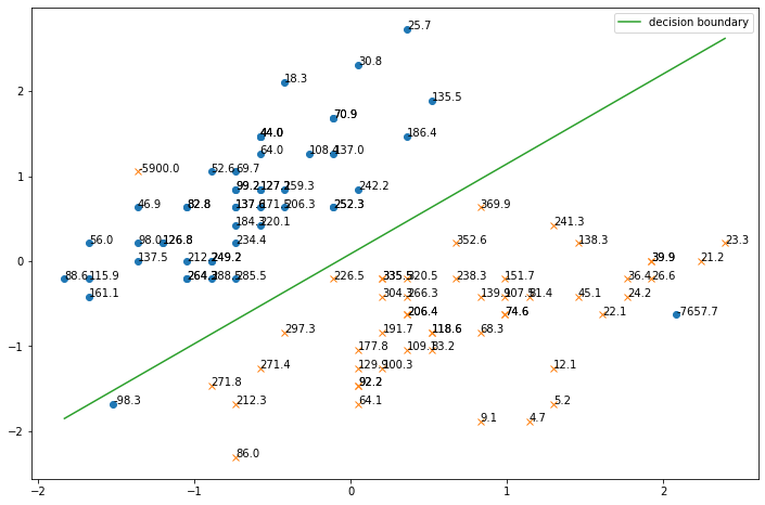
ミスラベルのサンプルのinfluence値が非常に高くなっていることがわかります．

また，左下のサンプルが決定境界をはみ出ていて，ミスラベルが学習に悪影響を及ぼしていることが懸念されます．

まとめ

influence関数を使うことで，決定境界に近い（自信のない）サンプルや，ミスラベルを見出すことができる．

Influence functionをロジスティック回帰に適用する

influence functionとは

ロジスティック回帰とinfluence function

ミスラベルを意図的に混入させた場合

まとめ