
この記事は現代化学(東京化学同人)の2022年4月号から2024年3月号まで連載された安藤耕司先生の「Pythonによる化学シミュレーション入門」を読んでやってみた記事です。詳しい内容は上記の「Pythonによる化学シミュレーション入門」をご参照ください。今回は、2023年2月号の古典力学(4)単振動の内容です。
単振動
単振動とはバネに繋がれた球の運動です。球の位置と速度は時間の関数で表されます。つまり、時間に依存する現象です。化学におけるシミュレーションは時間に依存する現象と時間に依存しない現象(つまり定常状態)の計算に大きく分けることができます。化学でよく扱う時間に依存する現象のシミュレーションはスペクトル解析や分子動力学計算などがあります。単振動は、この時間に依存する現象の一番簡単な例です。今回は、単振動を数値的に解析していきます。
方程式を立てる
古典力学の定法に沿って単振動の運動を解析しましょう。運動する球について、(1)運動方程式と(2)エネルギー保存則から式を導出します。
(1)運動方程式
$m\frac{d^2 x}{dt}= F = -kx$です。今回はこれを数値的に解析するのですが、ニ階微分は数値計算では扱いにくいので次のように2つの一階微分の式に分離します。
\begin{aligned}
\begin{cases}
  \frac{dx(t)}{dt} = v(t)\\
  \frac{dv(t)}{dt} = -\frac{k}{m}x(t)
\end{cases}
\end{aligned}
(2)エネルギー保存則
単振動では、運動エネルギーが$K = \frac{1}{2}mv^2$、ポテンシャルエネルギーが$F = - \frac{dV(x)}{dx}$です。このとき、次式のようなエネルギー保存が成り立ちます。
\frac{dE}{dt} = \frac{d(K+V)}{dt} = 0
解析解
先に解析解を示します。単振動の運動方程式$m\frac{d^2 x}{dt} = -kx$を解けば良いです。$\omega = \sqrt{\frac{k}{m}}$とすると、位置と速度の解析解は以下となります。
\begin{aligned}
\begin{cases}
  x(t) = \frac{v(0)}{\omega}\sin\omega t + x(0)\cos \omega t\\
  v(t) = v(0)\cos\omega t - x(0)\omega\sin \omega t
\end{cases}
\end{aligned}
これを次のようにプロットしてみます。
import numpy as np
import matplotlib.pyplot as plt

k, m = 1, 1
tmax, h = 20, 0.1

t0, x0, v0 = 0, 3, 0

t = np.arange(0, tmax, h)

omega = np.sqrt(k/m)

x = v0/omega*np.sin(omega*t) + x0*np.cos(omega*t)
v = v0*np.cos(omega*t) - x0*omega*np.sin(omega*t)

t, x, v = map(np.array, [t, x, v])

# plot
fig = plt.figure()
ax1 = fig.add_subplot(111)
ax1.plot(t,x, label="x")
ax1.set_ylabel("x")
ax1.set_xlabel("t")
ax2 = ax1.twinx()
ax2.plot(t,v,color="orange", label="v")
ax2.set_ylabel("v")
h1, l1 = ax1.get_legend_handles_labels()
h2, l2 = ax2.get_legend_handles_labels()
ax1.legend(h1+h2, l1+l2)
plt.show()

plt.plot(x,v)
plt.xlabel("x")
plt.ylabel("v")
plt.show()

ke = 0.5*m*np.array(v)**2
pe = 0.5*k*np.array(x)**2

plt.plot(t,ke, label="ke")
plt.plot(t,pe, label="pe")
plt.plot(t,ke + pe, label="ke+pe")
plt.legend()
plt.xlabel("t")
plt.ylabel("energy")
plt.show()
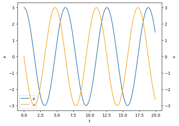
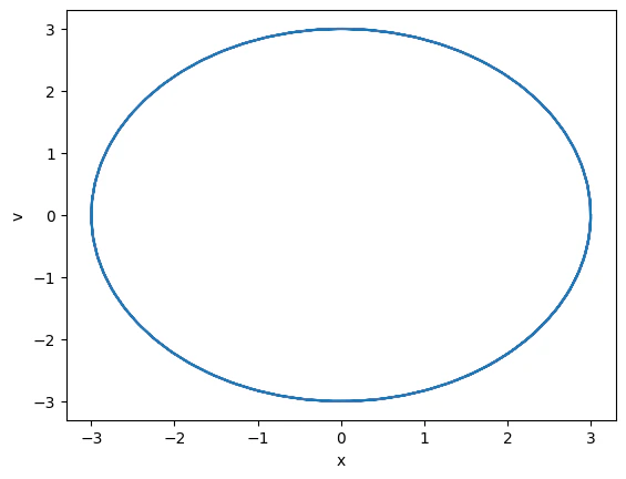
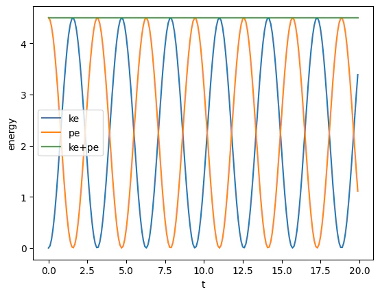
位置と速度が振動しています。位置を横軸、速度を縦軸に取ると閉曲線の楕円を描きます。エネルギーをプロットすると全エネルギーが保存していることがわかります。
微分方程式の数値解法
さて、単振動は解析解が簡単に解けますが、すべての運動において解析解が得られるわけではありません。その場合、微分方程式を数値的に解きます。以下、種々の数値的解法で単振動のシミュレーションをしていきます。
陽的オイラー法
まず、単振動の位置と速度の関係は$\frac{dx(t)}{dt} = v(t)$となるのでした。数値的に解析するために、$\frac{dx(t)}{dt} \simeq \frac{x(t+h)-x(t)}{h}$を用いて、微分を差分の式にすると、$x(t+h) = x(t) + v(t)h$と式変形できます。同様に、速度の微分を差分にすると、単振動の運動方程式は次の2つの式に変形できます。
\begin{aligned}
\begin{cases}
  x(t+h) = x(t) + v(t)h\\
  v(t+h) = v(t) + a(t)h = v(t) - \frac{kx(t)}{m}h
\end{cases}
\end{aligned}
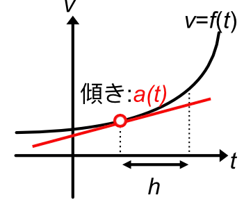
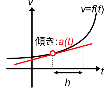
ここで、$a(t) = - \frac{kx(t)}{m}$を用いました。以下の図のように、$a(t)$は微分の区間の始点の傾きを代表して用いています。このような方法を陽的オイラー法と言います。
これを実装してプロットしてみます。
# 陽的オイラー法 (一次のルンゲ・クッタ法)

import numpy as np
import matplotlib.pyplot as plt

k, m = 1, 1
tmax, h = 20, 0.1

tt, xt, vt = 0, 3, 0
t, x, v = [], [], []

while tt <= tmax:
  t.append(tt)
  x.append(xt)
  v.append(vt)

  tt = tt + h
  xt1, vt1, = xt, vt

  xt = xt + vt*h
  vt = vt + (-k*xt1/m)*h

t, x, v = map(np.array, [t, x, v])

# plot
fig = plt.figure()
ax1 = fig.add_subplot(111)
ax1.plot(t,x, label="x")
ax1.set_ylabel("x")
ax1.set_xlabel("t")
ax2 = ax1.twinx()
ax2.plot(t,v,color="orange", label="v")
ax2.set_ylabel("v")
h1, l1 = ax1.get_legend_handles_labels()
h2, l2 = ax2.get_legend_handles_labels()
ax1.legend(h1+h2, l1+l2)
plt.show()

plt.plot(x,v)
plt.xlabel("x")
plt.ylabel("v")
plt.show()

ke = 0.5*m*np.array(v)**2
pe = 0.5*k*np.array(x)**2

plt.plot(t,ke, label="ke")
plt.plot(t,pe, label="pe")
plt.plot(t,ke + pe, label="ke+pe")
plt.legend()
plt.xlabel("t")
plt.ylabel("energy")
plt.show()
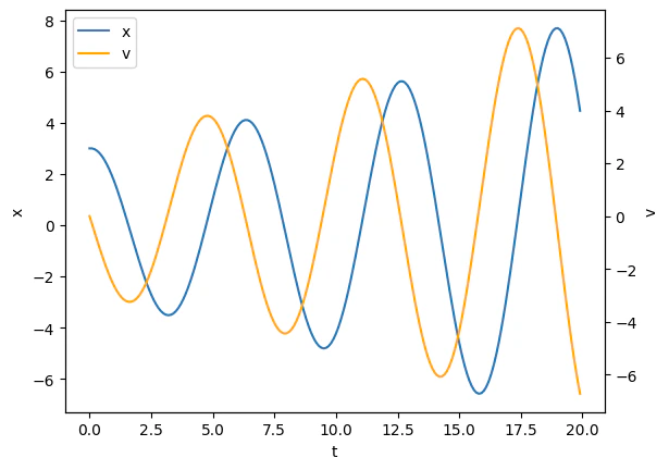
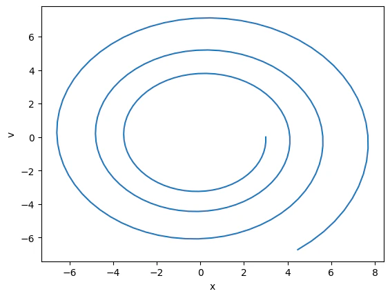
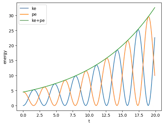
結果は、$x(t)$と$v(t)$、エネルギーは発散していき、計算結果がおかしくなります。これは実装を間違えたのではく、$a(t)$を用いていることの解析解からのズレです。オイラー法は反応速度のシミュレーションのようの単純な系では有用ですが、単振動では解析解からのずれが顕著です。
陰的オイラー法
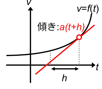
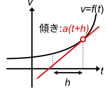
今度は、以下の図のように、微分の区間の終点の傾きを代表して用いてみます。このような方法を陰的オイラー法と言います。
# 陰的オイラー法

import numpy as np
import matplotlib.pyplot as plt

k, m = 1, 1
tmax, h = 20, 0.1

tt, xt, vt = 0, 3, 0
t, x, v = [], [], []

while tt <= tmax:
  t.append(tt)
  x.append(xt)
  v.append(vt)

  tt = tt + h

  xt = (xt + vt*h)/(1+(h**2)*k/m)
  vt = vt + (-k*xt/m)*h

t, x, v = map(np.array, [t, x, v])

# plot
fig = plt.figure()
ax1 = fig.add_subplot(111)
ax1.plot(t,x, label="x")
ax1.set_ylabel("x")
ax1.set_xlabel("t")
ax2 = ax1.twinx()
ax2.plot(t,v,color="orange", label="v")
ax2.set_ylabel("v")
h1, l1 = ax1.get_legend_handles_labels()
h2, l2 = ax2.get_legend_handles_labels()
ax1.legend(h1+h2, l1+l2)
plt.show()

plt.plot(x,v)
plt.xlabel("x")
plt.ylabel("v")
plt.show()

ke = 0.5*m*np.array(v)**2
pe = 0.5*k*np.array(x)**2

plt.plot(t,ke, label="ke")
plt.plot(t,pe, label="pe")
plt.plot(t,ke + pe, label="ke+pe")
plt.legend()
plt.xlabel("t")
plt.ylabel("energy")
plt.show()
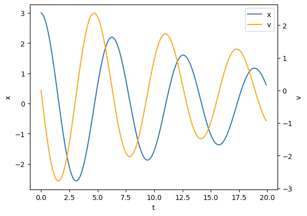
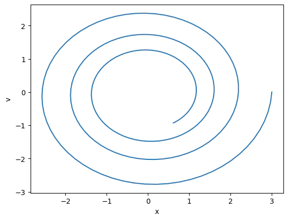
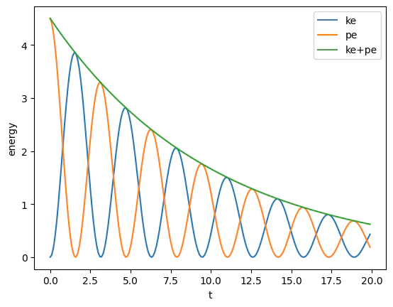
結果は先ほどとは逆で、$x(t)$と$v(t)$、エネルギーは収束していきます。
二次のルンゲ・クッタ法 (中点法)
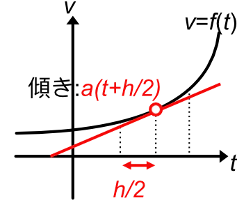
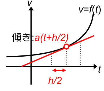
では、以下の図のように、微分の区間の中点の傾き$a(t+\frac{h}{2})$を用いてみます。このような方法を二次のルンゲ・クッタ法の中点法と言います。
# 二次のルンゲ・クッタ法(中点法)

import numpy as np
import matplotlib.pyplot as plt

k, m = 1, 1
tmax, h = 500, 0.1

tt, xt, vt = 0, 3, 0
t, x, v = [], [], []

while tt <= tmax:
  t.append(tt)
  x.append(xt)
  v.append(vt)

  tt = tt + h

  xt1, vt1 = xt, vt

  kx1 = vt1
  kv1 = -k * xt1 / m

  x_mid = xt1 + 0.5 * h * kx1
  v_mid = vt1 + 0.5 * h * kv1

  kx2 = v_mid
  kv2 = -k * x_mid / m

  xt = xt1 + h * kx2
  vt = vt1 + h * kv2

t, x, v = map(np.array, [t, x, v])

# plot
fig = plt.figure()
ax1 = fig.add_subplot(111)
ax1.plot(t,x, label="x")
ax1.set_ylabel("x")
ax1.set_xlabel("t")
ax2 = ax1.twinx()
ax2.plot(t,v,color="orange", label="v")
ax2.set_ylabel("v")
h1, l1 = ax1.get_legend_handles_labels()
h2, l2 = ax2.get_legend_handles_labels()
ax1.legend(h1+h2, l1+l2)
plt.show()

plt.plot(x,v)
plt.xlabel("x")
plt.ylabel("v")
plt.show()

ke = 0.5*m*np.array(v)**2
pe = 0.5*k*np.array(x)**2

plt.plot(t,ke, label="ke")
plt.plot(t,pe, label="pe")
plt.plot(t,ke + pe, label="ke+pe")
plt.legend()
plt.xlabel("t")
plt.ylabel("energy")
plt.show()
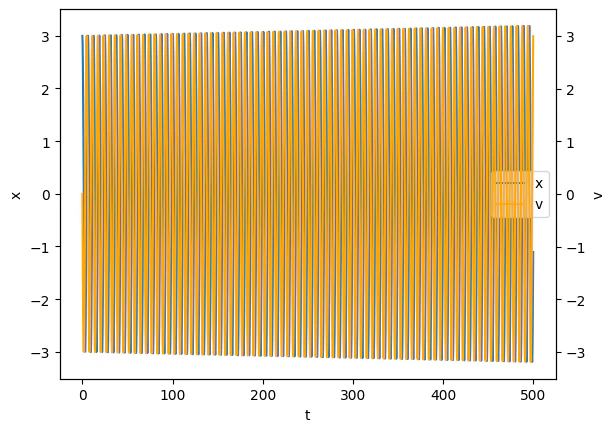
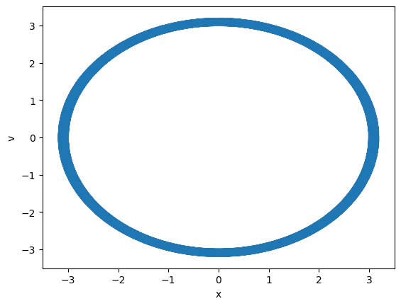

オイラー法に比べて解析解からのずれが小さくなります。しかし、ステップ数が増えるとやはり周期性を再現しなくなります。
二次のルンゲ・クッタ法(ヘルン法)
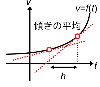
二次のルンゲ・クッタ法には、微分の区間の始点と終点の傾きの平均を取る方法もあります。このような方法を二次のルンゲ・クッタ法のヘルン法と言います。
# 二次のルンゲ・クッタ法 (ヘルン法)

import numpy as np
import matplotlib.pyplot as plt

k, m = 1, 1
tmax, h = 500, 0.1

tt, xt, vt = 0, 3, 0
t, x, v = [], [], []

while tt <= tmax:
  t.append(tt)
  x.append(xt)
  v.append(vt)

  tt = tt + h

  xt1, vt1 = xt, vt

  xs1 = vt1
  vs1 = -k * xt1 / m

  xt2 = xt1 + xs1 * h
  vt2 = vt1 + vs1 * h

  xs2 = vt2
  vs2 = -k * xt2 / m

  xt = xt1 + h * (xs1 + xs2) / 2
  vt = vt1 + h * (vs1 + vs2) / 2

t, x, v = map(np.array, [t, x, v])

# plot
fig = plt.figure()
ax1 = fig.add_subplot(111)
ax1.plot(t,x, label="x")
ax1.set_ylabel("x")
ax1.set_xlabel("t")
ax2 = ax1.twinx()
ax2.plot(t,v,color="orange", label="v")
ax2.set_ylabel("v")
h1, l1 = ax1.get_legend_handles_labels()
h2, l2 = ax2.get_legend_handles_labels()
ax1.legend(h1+h2, l1+l2)
plt.show()

plt.plot(x,v)
plt.xlabel("x")
plt.ylabel("v")
plt.show()

ke = 0.5*m*np.array(v)**2
pe = 0.5*k*np.array(x)**2

plt.plot(t,ke, label="ke")
plt.plot(t,pe, label="pe")
plt.plot(t,ke + pe, label="ke+pe")
plt.legend()
plt.xlabel("t")
plt.ylabel("energy")
plt.show()
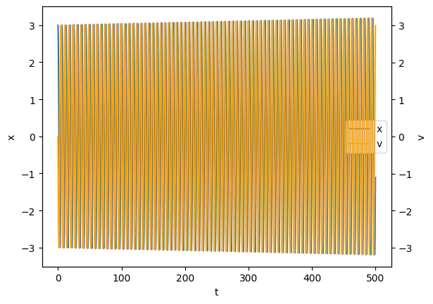
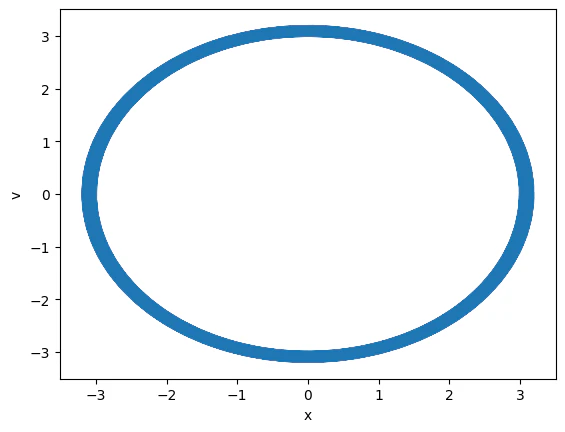
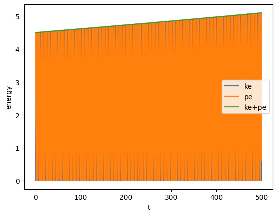
単振動に対しては中点法とヘルン法は似た結果になります。
一次のシンプレティック法
上記の数値解法に対して保存系の構造を保つように解析を行うのがシンプレティック法です。単振動におけるシンプレティック法を天下り的に受け入れると、次のようになります。
\begin{aligned}
\begin{cases}
  x(t+h) = x(t) + v(t)h\\
  v(t+h) = v(t) + a(t+h)h
\end{cases}
\end{aligned}
# 一次のシンプレティック法

import numpy as np
import matplotlib.pyplot as plt

k, m = 1, 1
tmax, h = 20, 0.1

tt, xt, vt = 0, 3, 0
t, x, v = [], [], []

while tt <= tmax:
  t.append(tt)
  x.append(xt)
  v.append(vt)

  tt = tt + h
  xt = xt + vt*h
  vt = vt + (-k*xt/m)*h

t, x, v = map(np.array, [t, x, v])

# plot
fig = plt.figure()
ax1 = fig.add_subplot(111)
ax1.plot(t,x, label="x")
ax1.set_ylabel("x")
ax1.set_xlabel("t")
ax2 = ax1.twinx()
ax2.plot(t,v,color="orange", label="v")
ax2.set_ylabel("v")
h1, l1 = ax1.get_legend_handles_labels()
h2, l2 = ax2.get_legend_handles_labels()
ax1.legend(h1+h2, l1+l2)
plt.show()

plt.plot(x,v)
plt.xlabel("x")
plt.ylabel("v")
plt.show()

ke = 0.5*m*np.array(v)**2
pe = 0.5*k*np.array(x)**2

plt.plot(t,ke, label="ke")
plt.plot(t,pe, label="pe")
plt.plot(t,ke + pe, label="ke+pe")
plt.legend()
plt.xlabel("t")
plt.ylabel("energy")
plt.show()
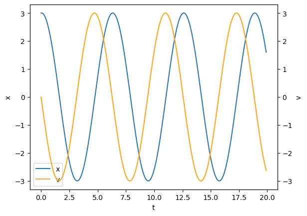
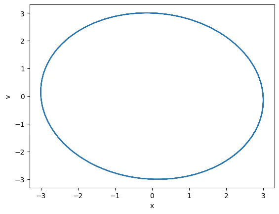
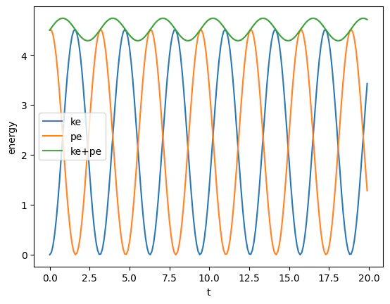
解析解と同様に、位置と速度が振動しています。位置を横軸、速度を縦軸に取ると閉曲線の楕円を描きます。エネルギーをプロットすると全エネルギーが振動してしまいますが、発散や収束はしなくなりました。
二次のシンプレティック法
最後にシンプレティック法においても、中点法のように計算をする際に$\frac{h}{2}$だけ時間をすすめると精度が向上しそうです。式で書き下すとこんな感じ。
\begin{aligned}
\begin{cases}
  x(t+0.5h) = x(t) + v(t)0.5h\\
  v(t+h) = v(t) + a(t+0.5h)h\\
  x(t+h) = x(t+0.5h) + v(t+h)0.5h
\end{cases}
\end{aligned}
# 二次のシンプレテック数値積分

import numpy as np
import matplotlib.pyplot as plt

k, m = 1, 1
tmax, h = 500, 0.1

tt, xt, vt = 0, 3, 0
t, x, v = [], [], []

while tt <= tmax:
  t.append(tt)
  x.append(xt)
  v.append(vt)

  tt = tt + h

  xt = xt + vt*(0.5*h)
  vt = vt + (-k*xt/m)*h
  xt = xt + vt*(0.5*h)

t, x, v = map(np.array, [t, x, v])

# plot
fig = plt.figure()
ax1 = fig.add_subplot(111)
ax1.plot(t,x, label="x")
ax1.set_ylabel("x")
ax1.set_xlabel("t")
ax2 = ax1.twinx()
ax2.plot(t,v,color="orange", label="v")
ax2.set_ylabel("v")
h1, l1 = ax1.get_legend_handles_labels()
h2, l2 = ax2.get_legend_handles_labels()
ax1.legend(h1+h2, l1+l2)
plt.show()

plt.plot(x,v)
plt.xlabel("x")
plt.ylabel("v")
plt.show()

ke = 0.5*m*np.array(v)**2
pe = 0.5*k*np.array(x)**2

plt.plot(t,ke, label="ke")
plt.plot(t,pe, label="pe")
plt.plot(t,ke + pe, label="ke+pe")
plt.legend()
plt.xlabel("t")
plt.ylabel("energy")
plt.show()
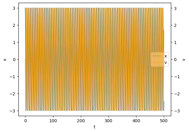
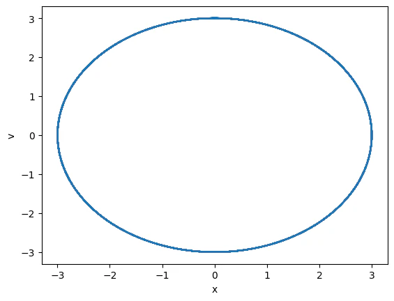
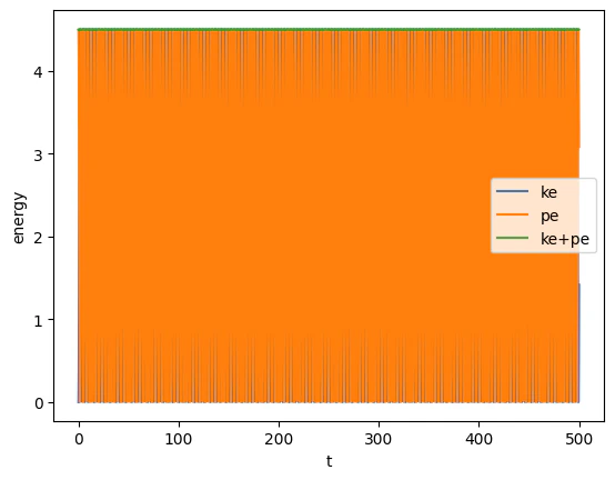
一次のシンプレテック法に比べてさらに精度の向上が見られます。
まとめ
以上、今回実施した微分方程式の数値解法をまとめます。
| 名称 | 特徴 | 数式 | 図 |
|---|---|---|---|
| 陽的オイラー法 | 区間の始点の傾きを使用 | $x(t+h) = x(t) + v(t)h$ $v(t+h) = v(t) + a(t)h$ |
 |
| 陰的オイラー法 | 区間の終点の傾きを使用 | $x(t+h) = x(t) + v(t+h)h$ $v(t+h) = v(t) + a(t+h)h$ |
 |
| 二次のルンゲ・クッタ法(中点法) | 区間の中点の傾きを使用 | $x(t+h) = x(t) + v(t+h)h$ $v(t+h) = v(t) + a(t+\frac{h}{2})h$ |
 |
| 二次のルンゲ・クッタ法(ヘルン法) | 区間の両端の平均の傾きを使用 | $x(t+h) = x(t) + \frac{v(t) + v_{temp}}{2}h$ $v(t+h) = v(t) + \frac{a(t) + a_{temp}}{2}h$ |
 |
| 一次のシンプレティック法 | 保存系の構造を保つ | $x(t+h) = x(t) + v(t)h$ $v(t+h) = v(t) + a(t+h)h$ |
|
| 二次のシンプレティック法 | 保存系の構造を二次精度で保つ | $x(t+\frac{h}{2}) = x(t) + v(t)\frac{h}{2}$ $v(t+h) = v(t) + a(t+\frac{h}{2})h$ $x(t+h) = x(t+\frac{h}{2}) + v(t+h)\frac{h}{2}$ |
|
| 解析解 | 理論に厳密な解 |
連載記事目次
・「Pythonによる化学シミュレーション入門」をやってみたよ~単分子一次反応の反応速度論~
・「Pythonによる化学シミュレーション入門」をやってみたよ2~色々な反応の反応速度~
・「Pythonによる化学シミュレーション入門」をやってみたよ3~振動反応~
・「Pythonによる化学シミュレーション入門」をやってみたよ4~ランダムウォークと拡散現象~
・「Pythonによる化学シミュレーション入門」をやってみたよ5~ブラウン運動とランジュバン方程式~
・「Pythonによる化学シミュレーション入門」をやってみたよ6~分子軌道法(1)~