はじめに
機械学習において性能評価は欠かせない手順のひとつですが、
分類タスクにおける性能評価によく使われるのが、ROC曲線です。

PythonでROC曲線を描画するには、Scikit-Learnのplot_roc_curve(←Scikit-Learn1.2で削除されました)RocCurveDisplay.from_estimatorというメソッドを使用するのが一般的ですが、このメソッド、多クラス分類やクロスバリデーションでの描画が出来ない等、制約が多いです。
そこで今回、これらの制約をクリアすべく、
・多クラス分類のROC曲線描画
・クロスバリデーションのROC曲線描画
を実現するライブラリを作成しました。
本機能はこちらの記事で紹介したseaborn-analyzerライブラリに、plot_roc_curve_multiclass()メソッドおよびroc_plot()メソッドとして追加しております。
本ツールを有用だと感じられたら、GitHubにスター頂けると有難いです!
インストール方法
インストールは以下のようにpipから行います
pip install seaborn-analyzer
使用法
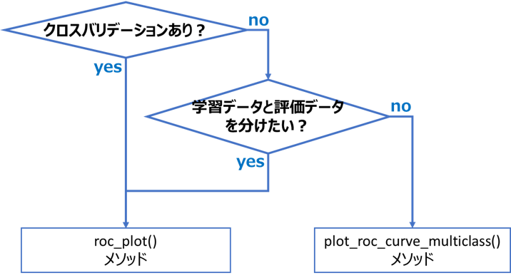
plot_roc_curve_multiclass()メソッドとroc_plot()メソッドの使い分けは、以下のフローにより判断してください
多クラス分類のROC曲線描画
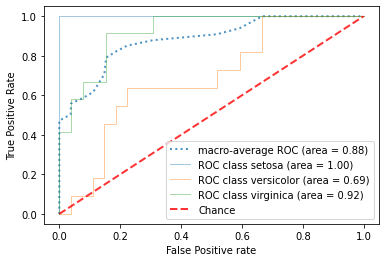
多クラス分類でのROC曲線描画は、plot_roc_curve_multiclass()メソッドで実行します
(学習データと評価データを分けない場合、後述のroc_plot()メソッドでも描画可能)
import seaborn as sns
from sklearn.svm import SVC
from sklearn.model_selection import train_test_split
import numpy as np
import matplotlib.pyplot as plt
from seaborn_analyzer import classplot
# Load dataset
iris = sns.load_dataset("iris")
OBJECTIVE_VARIALBLE = 'species'  # 目的変数
USE_EXPLANATORY = ['petal_width', 'petal_length', 'sepal_width', 'sepal_length']  # 説明変数
y = iris[OBJECTIVE_VARIALBLE].values
X = iris[USE_EXPLANATORY].values
# ノイズ追加(ROC曲線を見やすくするための処理。実使用時は実施しないで下さい)
random_state = np.random.RandomState(0)
n_samples, n_features = X.shape
X = np.c_[X, random_state.randn(n_samples, 10 * n_features)]
# ROC曲線描画
X_train, X_test, y_train, y_test = train_test_split(X, y, shuffle=True, random_state=42)
estimator = SVC(probability=True, random_state=42)
classplot.plot_roc_curve_multiclass(estimator, X_train, y_train,
                                    X_test=X_test, y_test=y_test)
plt.plot([0, 1], [0, 1], label='Chance', alpha=0.8,
         lw=2, color='red', linestyle='--')
plt.legend(loc='lower right')
引数一覧はGitHubの該当項目を、機能詳細は後述の機能解説を参照ください。
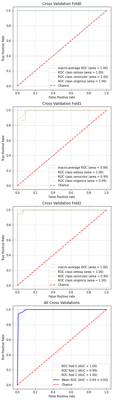
クロスバリデーションでのROC曲線描画
クロスバリデーションでのROC曲線描画は、roc_plot()メソッドで実行します。
本メソッドは内部でplot_roc_curve_multiclass()メソッドを呼び出しているので、「クロスバリデーションかつ多クラス分類」のROC曲線も描画可能です。
from lightgbm import LGBMClassifier
import seaborn as sns
import matplotlib.pyplot as plt
from seaborn_analyzer import classplot
# Load dataset
iris = sns.load_dataset("iris")
OBJECTIVE_VARIALBLE = 'species' # 目的変数
USE_EXPLANATORY = ['petal_width', 'petal_length', 'sepal_width', 'sepal_length'] # 説明変数
y = iris[OBJECTIVE_VARIALBLE].values
X = iris[USE_EXPLANATORY].values
fit_params = {'verbose': 0,
'early_stopping_rounds': 10,
'eval_metric': 'rmse',
'eval_set': [(X, y)]
}
# ROC曲線描画
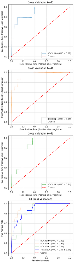
estimator = LGBMClassifier(random_state=42, n_estimators=10000)
fig, axes = plt.subplots(4, 1, figsize=(6, 24))
classplot.roc_plot(estimator, X, y, ax=axes, cv=3, fit_params=fit_params)
引数一覧はGitHubの該当項目を、機能詳細は後述の機能解説を参照ください。
必要要件
本ツールには以下のライブラリが必要となります
Python >=3.6
Numpy >=1.20.3
Pandas >=1.2.4
Matplotlib >=3.3.4
Seaborn >=0.11.0
Scipy >=1.6.3
Scikit-learn >=0.24.2
機能解説
本ライブラリの描画対象であるROC曲線の意味と、ライブラリで実現できる機能を解説します。
ROC曲線とは?
機械学習の分類タスク(2クラス分類)では、PositiveクラスとNegativeクラスを分類します。この分類結果の正誤を集計したものが、下図の混同行列です
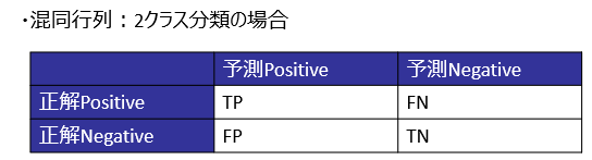
この混同行列において、見すぎ(FPが多い)と見逃し(FNが多い)はトレードオフ関係にあり、片方が良化すると基本的にはもう片方が悪化します。
このようなトレードオフ関係を可視化し、性能を評価するためのグラフが、ROC曲線です。
(参考)

ROC曲線は、閾値を変えた際の、TPR(見逃しの少なさ)とFPR(見すぎの多さ)の変化をプロットした曲線です。
Scikit-Learnにおいては、学習器からクラス確率を求め、その閾値を離散的に変化させた際のTPR、FPRを求めて線でつなぐことで、ROC曲線を描画します。
RocCurveDisplay.from_estimator()メソッドの制約
先ほど、「Scikit-LearnのRocCurveDisplay.from_estimator()メソッドは制約が多い」と言いましたが、実用上は以下の3点が問題となります
1. クロスバリデーションでは使えない
2. 多クラス分類では使えない
3. fit_paramsを渡せない
詳細と本ツールでの解決策を下記します
制約の内容と解決策
上記1~3の制約の内容と、どのように解決したかを詳説します
制約1. クロスバリデーション時のROC曲線が描画できない
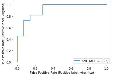
RocCurveDisplay.from_estimator()メソッドは、学習済の分類器を渡して実行するため、以下のような1本のROC曲線のみを描画することができます
import seaborn as sns
from sklearn.svm import SVC
from sklearn.model_selection import train_test_split
from sklearn.metrics import RocCurveDisplay
import numpy as np
# Load dataset
iris = sns.load_dataset("iris")
iris = iris[iris['species'] != 'setosa']
OBJECTIVE_VARIALBLE = 'species'  # 目的変数
USE_EXPLANATORY = ['petal_width', 'petal_length', 'sepal_width', 'sepal_length']  # 説明変数
y = iris[OBJECTIVE_VARIALBLE].values
X = iris[USE_EXPLANATORY].values
# ノイズ追加(ROC曲線を見やすくするため)
random_state = np.random.RandomState(0)
n_samples, n_features = X.shape
X = np.c_[X, random_state.randn(n_samples, 10 * n_features)]
# ROC曲線描画
X_train, X_test, y_train, y_test = train_test_split(X, y, shuffle=True, random_state=42)
estimator = SVC(probability=True, random_state=42)
estimator.fit(X_train, y_train)
RocCurveDisplay.from_estimator(estimator, X_test, y_test)
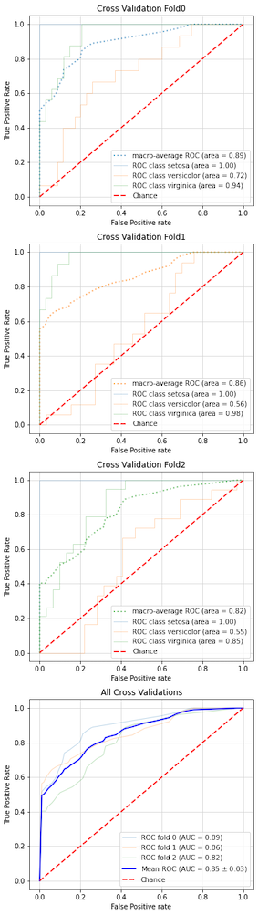
以下のようなクロスバリデーション時のROC曲線(FoldごとのROC曲線+平均ROC曲線)を描画することはできません。
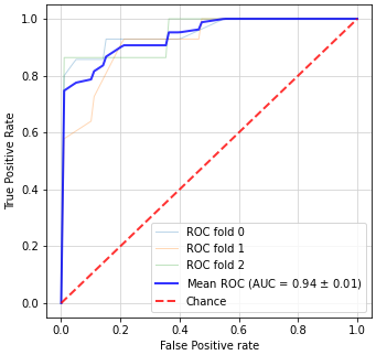
分類の性能評価にはクロスバリデーションを使う事が多いので、これが可視化できない事は大きな問題です。
解決策
scikit-learnでの解説記事を参考に、クロスバリデーションでのROC曲線描画機能を実装し、ライブラリ中のroc_plot()メソッドに組み込みました。
cv引数にクロスバリデーション用のインスタンスを渡すことで、以下のようにクロスバリデーションでのROC曲線描画を実現できます
(cv引数に数値を指定すれば、指定した数でKFold分割します)
from sklearn.svm import SVC
from sklearn.model_selection import KFold
import seaborn as sns
import matplotlib.pyplot as plt
from seaborn_analyzer import classplot
import numpy as np
# Load dataset
iris = sns.load_dataset("iris")
iris = iris[iris['species'] != 'setosa']
OBJECTIVE_VARIALBLE = 'species'  # 目的変数
USE_EXPLANATORY = ['petal_width', 'petal_length', 'sepal_width', 'sepal_length']  # 説明変数
y = iris[OBJECTIVE_VARIALBLE].values
X = iris[USE_EXPLANATORY].values
# ノイズ追加(ROC曲線を見やすくするため)
random_state = np.random.RandomState(0)
n_samples, n_features = X.shape
X = np.c_[X, random_state.randn(n_samples, 10 * n_features)]
# ROC曲線描画
estimator = SVC(probability=True, random_state=42)
fig, axes = plt.subplots(4, 1, figsize=(6, 24))
cv = KFold(n_splits=3, shuffle=True, random_state=42)
classplot.roc_plot(estimator, X, y, ax=axes, cv=cv)
制約2. 多クラス分類でのROC曲線が描画できない
各クラスごとに、残りのクラスをひとまとめにした2クラス分類(One vs Rest, OVRと言います。こちらが分かりやすいです)を実施し、それぞれ求めた混同行列から、TPRの平均値を求めます(横軸となるFPRは最初に定めた固定値のリストを使用)。
平均の求め方は、以下のミクロ平均とマクロ平均があります。
ミクロ平均
クラスごとのデータ数で重みづけしたTPRとFPRの平均を求めます。
以下の式で求められます。
TPR_{micro} = \frac{\sum_{i=1}^{n} TP_i}{\sum_{i=1}^{n} TP_i+\sum_{i=1}^{n} FN_i}
FPR_{micro} = \frac{\sum_{i=1}^{n} FP_i}{\sum_{i=1}^{n} FP_i+\sum_{i=1}^{n} TN_i}
マクロ平均
クラスごとに求めたTPRをそのまま平均します
クラスごとの添字をi、クラス数をnで表すと、以下のように求められます
TPR_{macro} = \frac{\sum_{i=1}^{n} TPR_i}{n} = \frac{\sum_{i=1}^{n} \frac{TP_i}{TP_i+FN_i}}{n}
FPR_{macro} = \frac{\sum_{i=1}^{n} FPR_i}{n} = \frac{\sum_{i=1}^{n} \frac{FP_i}{FP_i+TN_i}}{n}
クラスごとのTPRを求める際にFPRの値を揃えておけば、TPRのマクロ平均だけを求めればよくなり、計算が楽になります(Scikit-Learnでもこのような求め方をしているようです)
ミクロ平均とマクロ平均の使い分け
ミクロ平均とマクロ平均の使い分けは、以下のようになります
| 用途 | 選択する平均法 |
|---|---|
| データ数の少ないクラスを重視したい場合 | マクロ平均 |
| データ数の多いクラスを重視したい場合 | ミクロ平均 |
詳細はこちらやこちらが詳しいですが、クラスごとにデータ数の偏りが大きい不均衡データにおいては、小さいクラスの影響を大きく評価するmacroの方がmicroより良いと言われています。
(逆に、大きなクラスさえ正解していれば小さいクラスでの性能は問わない、という場合はf1_microを選択するのも可です)
問題と解決策
前置きが長くなりましたが、RocCurveDisplay.from_estimatorメソッドには上記のようなミクロ平均、マクロ平均を求める機能は存在せず、多クラス分類でのROC曲線を描画できません(エラーが出ます)
機械学習の可視化ライブラリYellowBrickや、これを利用したPyCaretではミクロ平均やマクロ平均のROC曲線を描画できますが、これらを利用すると前述のクロスバリデーションや後述のfit_paramsを適用する事が困難となるため、やはり課題は残ります。
そこでこちらのScikit-Learnの記事
を参考に多クラス分類でのROC曲線描画機能を組み込んだ、plot_roc_curve_multiclass()メソッドを実装しました
import seaborn as sns
from sklearn.svm import SVC
from sklearn.model_selection import train_test_split
import numpy as np
import matplotlib.pyplot as plt
from seaborn_analyzer import classplot
# Load dataset
iris = sns.load_dataset("iris")
OBJECTIVE_VARIALBLE = 'species'  # 目的変数
USE_EXPLANATORY = ['petal_width', 'petal_length', 'sepal_width', 'sepal_length']  # 説明変数
y = iris[OBJECTIVE_VARIALBLE].values
X = iris[USE_EXPLANATORY].values
# ノイズ追加(ROC曲線を見やすくするため)
random_state = np.random.RandomState(0)
n_samples, n_features = X.shape
X = np.c_[X, random_state.randn(n_samples, 10 * n_features)]
# ROC曲線描画
X_train, X_test, y_train, y_test = train_test_split(X, y, shuffle=True, random_state=42)
estimator = SVC(probability=True, random_state=42)
classplot.plot_roc_curve_multiclass(estimator, X_train, y_train,
                                    X_test=X_test, y_test=y_test)
plt.plot([0, 1], [0, 1], label='Chance', alpha=0.8,
         lw=2, color='red', linestyle='--')
plt.legend(loc='lower right')

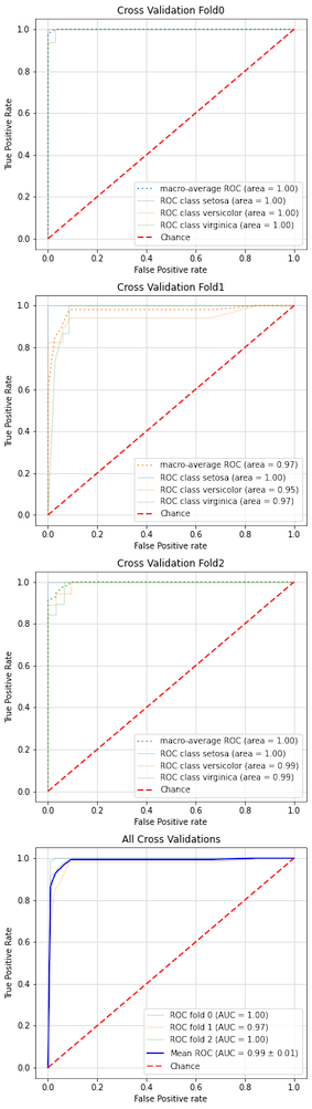
また、前述のroc_plot()メソッドを使用すれば、「多クラス分類かつクロスバリデーションでのROC曲線」を描画することも可能です
from sklearn.svm import SVC
import seaborn as sns
import matplotlib.pyplot as plt
from seaborn_analyzer import classplot
import numpy as np
# Load dataset
iris = sns.load_dataset("iris")
OBJECTIVE_VARIALBLE = 'species'  # 目的変数
USE_EXPLANATORY = ['petal_width', 'petal_length', 'sepal_width', 'sepal_length']  # 説明変数
y = iris[OBJECTIVE_VARIALBLE].values
X = iris[USE_EXPLANATORY].values
# ノイズ追加(ROC曲線を見やすくするため)
random_state = np.random.RandomState(0)
n_samples, n_features = X.shape
X = np.c_[X, random_state.randn(n_samples, 10 * n_features)]
# ROC曲線描画
estimator = SVC(probability=True, random_state=42)
fig, axes = plt.subplots(4, 1, figsize=(6, 24))
classplot.roc_plot(estimator, X, y, ax=axes, cv=3)
制約3. fit_paramsを渡せない
上記の多クラス分類でOVR学習器の作成に使用しているOneVsRestClassifierクラスは、学習時のfit()メソッドに引数(以下fit_paramsと呼びます)を渡すことができません。
これは、XGBoostやLightGBMで多用されるearly_stopping_roundが使用できないことを意味しており、これらのアルゴリズムを使用する際に大きな支障が出ます。
解決策
OneVsRestClassifierクラスを継承して、fit()メソッドを適用可能なOneVsRestClassifierPatchedクラスを作成しました(こちらのIssuesを参考にさせて頂きました)
ですのでplot_roc_curve_multiclass()メソッド、roc_plot()メソッド共に、fit_params引数にパラメータを渡せば、学習時に適用されます
from lightgbm import LGBMClassifier
import seaborn as sns
import matplotlib.pyplot as plt
from seaborn_analyzer import classplot
# Load dataset
iris = sns.load_dataset("iris")
OBJECTIVE_VARIALBLE = 'species'  # Objective variable
USE_EXPLANATORY = ['petal_width', 'petal_length', 'sepal_width', 'sepal_length']  # Explantory variables
y = iris[OBJECTIVE_VARIALBLE].values
X = iris[USE_EXPLANATORY].values
fit_params = {'verbose': 0,
              'early_stopping_rounds': 10,
              'eval_metric': 'multi_logloss',
              'eval_set': [(X, y)]
              }
# Plot ROC curve with cross validation in multiclass classification
estimator = LGBMClassifier(random_state=42, n_estimators=10000)
fig, axes = plt.subplots(4, 1, figsize=(6, 24))
classplot.roc_plot(estimator, X, y, ax=axes, cv=3, fit_params=fit_params)
ROC曲線の活用例:
ROC曲線を性能評価に使う事は、他の評価指標(LogLoss、Accuracy等)と比較して以下のようなメリットがあります。
・見すぎと見逃しのバランスを連続的に評価できる
・グラフで可視化できるため、直感的な理解の助けとなる
上記を踏まえて、ROC曲線の活用例を紹介します。
活用例1:見逃しに強いか、見すぎに強いかの確認
適切なデータセットが見付からなかったので実装例はありませんが、
以下の記事のように見すぎと見逃しどちらに強いモデルかの評価に使われることがあります。
上記の特性から、検査機のように見逃しを極力許容したくない用途(逆に見すぎは許容する)においては、見逃しに強いモデルを判断できるROC曲線はモデル選択や閾値決定の助けとなるでしょう。
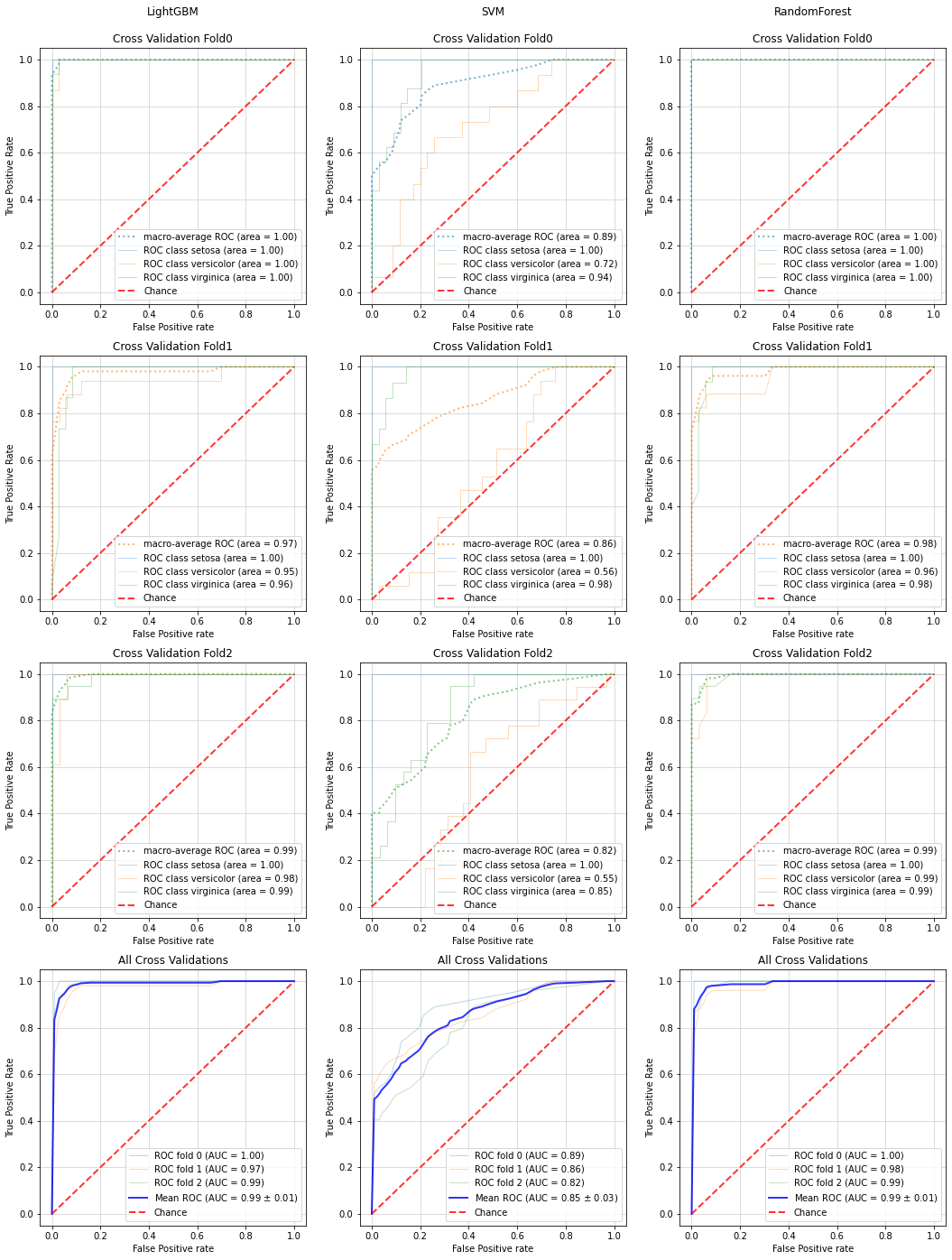
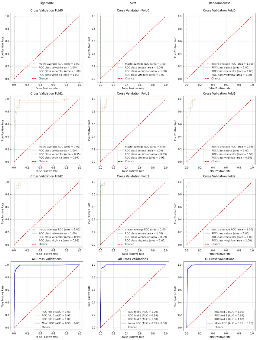
活用例2:ノイズへの強さ(余分な説明変数の追加に対する頑強さ)の比較
以下の例では、ノイズ列(ランダムに生成した意味を持たない説明変数)を元の列数の10倍加えた場合の、
・LightGBM
・SVM
・RandomForest
の3種類の分類器における、ROC曲線の変化をプロットしています。
ノイズ付加前
from sklearn.svm import SVC
from sklearn.ensemble import RandomForestClassifier
from lightgbm import LGBMClassifier
import seaborn as sns
import matplotlib.pyplot as plt
from seaborn_analyzer import classplot
# Load dataset
iris = sns.load_dataset("iris")
OBJECTIVE_VARIALBLE = 'species'  # Objective variable
USE_EXPLANATORY = ['petal_width', 'petal_length', 'sepal_width', 'sepal_length']  # Explantory variables
y = iris[OBJECTIVE_VARIALBLE].values
X = iris[USE_EXPLANATORY].values
fit_params = {'verbose': 0,
              'early_stopping_rounds': 10,
              'eval_metric': 'multi_logloss',
              'eval_set': [(X, y)]
              }
# Plot ROC curve with three classifiers
estimator1 = LGBMClassifier(random_state=42, n_estimators=10000)
estimator2 = SVC(probability=True, random_state=42)
estimator3 = RandomForestClassifier(random_state=42)
fig, axes = plt.subplots(4, 3, figsize=(18, 24))
ax_pred = [[row[i] for row in axes] for i in range(3)]
classplot.roc_plot(estimator1, X, y, ax=ax_pred[0], cv=3, fit_params=fit_params)
classplot.roc_plot(estimator2, X, y, ax=ax_pred[1], cv=3)
classplot.roc_plot(estimator3, X, y, ax=ax_pred[2], cv=3)
# Add etimator name to the graph
ax_pred[0][0].set_title(f'LightGBM\n\n{ax_pred[0][0].title._text}')
ax_pred[1][0].set_title(f'SVM\n\n{ax_pred[1][0].title._text}')
ax_pred[2][0].set_title(f'RandomForest\n\n{ax_pred[2][0].title._text}')
ノイズ付加後
# Load dataset
iris = sns.load_dataset("iris")
OBJECTIVE_VARIALBLE = 'species'  # Objective variable
USE_EXPLANATORY = ['petal_width', 'petal_length', 'sepal_width', 'sepal_length']  # Explantory variables
y = iris[OBJECTIVE_VARIALBLE].values
X = iris[USE_EXPLANATORY].values
# Add random noise features
random_state = np.random.RandomState(0)
n_samples, n_features = X.shape
X = np.c_[X, random_state.randn(n_samples, 10 * n_features)]
fit_params = {'verbose': 0,
              'early_stopping_rounds': 10,
              'eval_metric': 'multi_logloss',
              'eval_set': [(X, y)]
              }
# Plot ROC curve with three classifiers
estimator1 = LGBMClassifier(random_state=42, n_estimators=10000)
estimator2 = SVC(probability=True, random_state=42)
estimator3 = RandomForestClassifier(random_state=42)
fig, axes = plt.subplots(4, 3, figsize=(18, 24))
ax_pred = [[row[i] for row in axes] for i in range(3)]
classplot.roc_plot(estimator1, X, y, ax=ax_pred[0], cv=3, fit_params=fit_params)
classplot.roc_plot(estimator2, X, y, ax=ax_pred[1], cv=3)
classplot.roc_plot(estimator3, X, y, ax=ax_pred[2], cv=3)
# Add etimator name to the graph
ax_pred[0][0].set_title(f'LightGBM\n\n{ax_pred[0][0].title._text}')
ax_pred[1][0].set_title(f'SVM\n\n{ax_pred[1][0].title._text}')
ax_pred[2][0].set_title(f'RandomForest\n\n{ax_pred[2][0].title._text}')
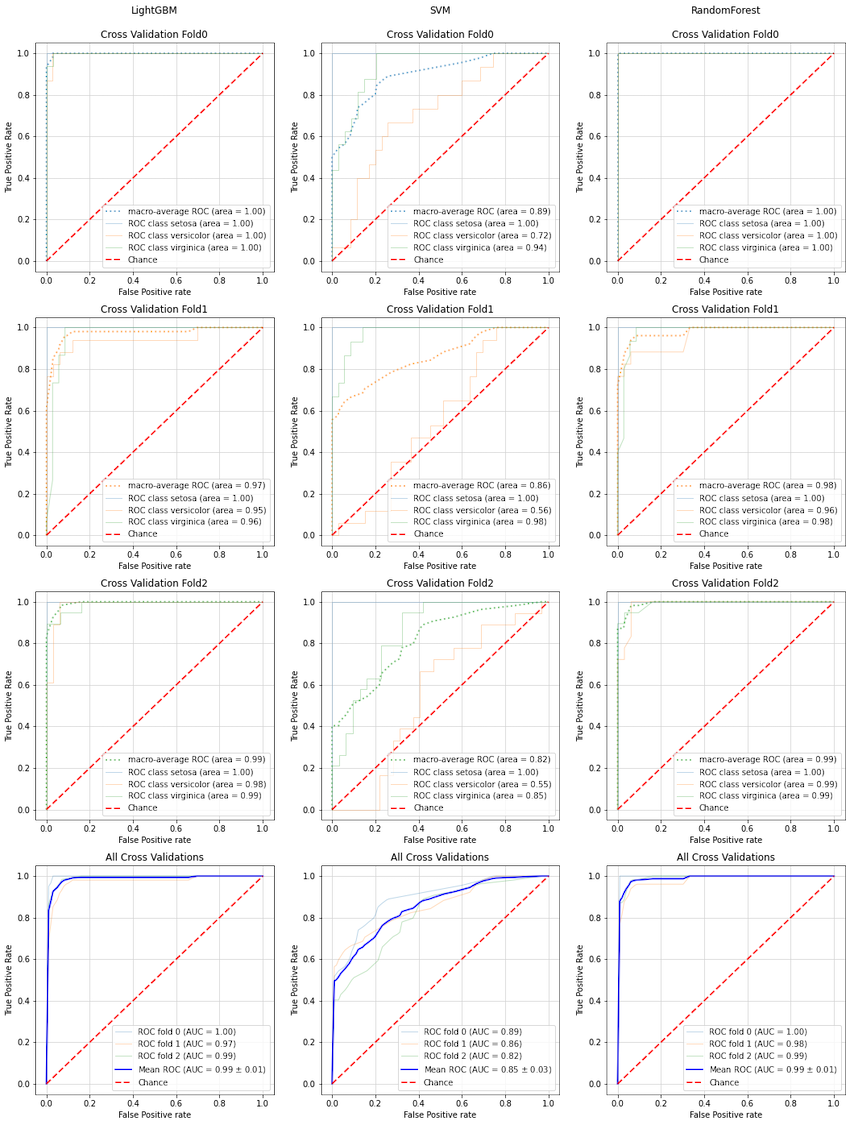
LightGBM、RandamForestはノイズ付加前後でROC曲線があまり変化していないのに対し、
SVMはノイズ付加によりROC曲線が大きく悪化していることが分かります。
現実のデータでは、上記ノイズ列のように目的変数にほぼ影響しない(意味のない)説明変数が大量に含まれている事例が多く、このようなデータでは特徴量選択をゴリゴリ頑張って変数を絞る必要があるのですが、上記ノイズ列評価の結果から、
・LightGBMやRandomForestは特徴量選択が不十分でも高い性能が出せる
・SVMは特徴量選択が不十分だと性能が落ちる
ことが分かります。
アルゴリズムの特性の違いをグラフで可視化できるので、ROC曲線の利便性が実感できたかと思います。