機械学習入門第三弾は、SVM(SuportVectorMachine)です。
K-means(K-近傍法)、 RFC(RandomForestClassification)、そしてSVMがクラス分類における機械学習御三家と言える手法だと思います。そこにDL(DeepLearning)が殴り込みをしたような構図です。
※【追記】K-meansとK-近傍法は、以下の参考の通り異なる手法でした。そのため本文も一部加筆修正しました
【参考】
・k近傍法とk平均法の違いと詳細
当面の目標
機械学習のクラス分類という面についてまとめます。
・K-meansクラスタリング
・ランダムフォレストでクラス分類
・SVMでクラス分類(今回の記事)
・DeepLearningでクラス分類
※DeepLearningは昨年集中してやりましたが、対比するためにまとめる予定です
今回やったこと
・SVM
・SVMでMNISTライクな手書き数字分類
・SVMでランダムフォレストに殴り込み;K-meansもランダムフォレストに殴り込みしました(追記)
・SVMでK-meansに殴り込み;参考だけ紹介しました(逆センスですが…)
・SVM
SVMの紹介的なアプリを動かしてみます。解説は省略します。
【参考】
・SVM(多クラス分類)
参考のアプリがまんま動きましたが、あんまりおもしろくないので、データ出力等少しだけ変更しました。
import numpy as np
import matplotlib.pyplot as plt
# %matplotlib inline
from sklearn import datasets
from sklearn.cross_validation import train_test_split # クロスバリデーション用
from sklearn.svm import SVC # SVM用
from sklearn import metrics       # 精度検証用
import pandas as pd

# データ用意
iris = datasets.load_iris()    # データロード
df = pd.DataFrame(iris.data, columns=iris.feature_names)
df['target'] = iris.target_names[iris.target] #これないと名前が出ない
# df.head() #これだけじゃ出力しない
print(df.head())

X = iris.data                  # 説明変数セット
Y = iris.target                # 目的変数セット
X_train, X_test, Y_train, Y_test = train_test_split(X, Y, random_state=0) # random_stateはseed値。
print(len(X_train),len(Y_train),len(X_test),len(Y_test))

# SVM実行
model = SVC()               # インスタンス生成
model.fit(X_train, Y_train) # SVM実行

# 予測実行
predicted = model.predict(X_test) # テストデータでの予測実行
acc=metrics.accuracy_score(Y_test, predicted)
print("acc=",acc)
これ実行すると、以下の警告がでますが、とりあえず以下の結果が得られます。
cross_validation.py:41: DeprecationWarning:...
   sepal length (cm)  sepal width (cm)  petal length (cm)  petal width (cm)  \
0                5.1               3.5                1.4               0.2
1                4.9               3.0                1.4               0.2
2                4.7               3.2                1.3               0.2
3                4.6               3.1                1.5               0.2
4                5.0               3.6                1.4               0.2

   target
0  setosa
1  setosa
2  setosa
3  setosa
4  setosa
112 112 38 38
acc= 0.973684210526
精度はまあまあですが、データ150個(学習112個、テスト38個)です。
※データ出力はpandas使っています。iris.head()だけだと出力できません
【参考】
・irisのデータセットをpandasで使う
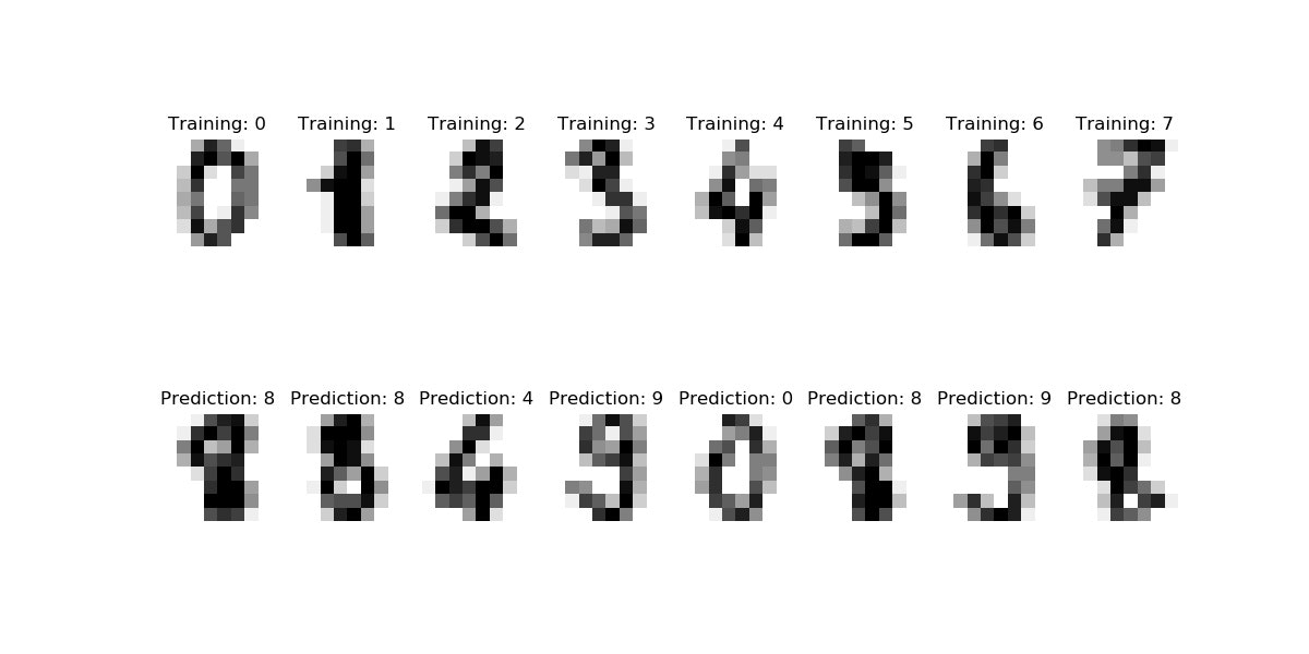
・SVMでMNISTライクな手書き数字分類
次は以下の参考を動かします。これもまんま動きました。
【参考】
・Recognizing hand-written digits
コードは、肝心なところだけ抜き出しますので、コメントは原文見てください。
また、少しだけ改変しています。
"""
================================
Recognizing hand-written digits
================================
"""
print(__doc__)
# Author: Gael Varoquaux <gael dot varoquaux at normalesup dot org>
# License: BSD 3 clause
import matplotlib.pyplot as plt
from sklearn import datasets, svm, metrics
digits = datasets.load_digits()

plt.figure(figsize=(12, 6)) #ここ追加しました
images_and_labels = list(zip(digits.images, digits.target))
for index, (image, label) in enumerate(images_and_labels[:8]): #4から8に変更
    plt.subplot(2, 8, index + 1)  #4から8に変更
    plt.axis('off')  #これコメントアウトすると枠と座標が出る
    plt.imshow(image, cmap=plt.cm.gray_r, interpolation='nearest')
    plt.title('Training: %i' % label)

# To apply a classifier on this data, we need to flatten the image, to
# turn the data in a (samples, feature) matrix:
n_samples = len(digits.images)
print('n_samples=',n_samples)
data = digits.images.reshape((n_samples, -1))

# Create a classifier: a Support Vector Classifier
classifier = svm.SVC(gamma=0.001)
# We learn the digits on the first half of the digits;学習データは前半半分
classifier.fit(data[:n_samples // 2], digits.target[:n_samples // 2])

# Now predict the value of the digit on the second half:Testデータは後半半分
expected = digits.target[n_samples // 2:]
predicted = classifier.predict(data[n_samples // 2:])

print("Classification report for classifier %s:\n%s\n"
      % (classifier, metrics.classification_report(expected, predicted)))
print("Confusion matrix:\n%s" % metrics.confusion_matrix(expected, predicted))

images_and_predictions = list(zip(digits.images[n_samples // 2:], predicted))
for index, (image, prediction) in enumerate(images_and_predictions[:8]):
    plt.subplot(2, 8, index + 9)
    plt.axis('off')
    plt.imshow(image, cmap=plt.cm.gray_r, interpolation='nearest')
    plt.title('Prediction: %i' % prediction)
plt.savefig('svm_mnistlike.jpg')
plt.pause(1)
実行例は以下のとおり、実行は瞬時に終わります。
サンプル数はn_samples= 1797です。
>python svm_mnistlike.py

================================
Recognizing hand-written digits
================================

n_samples= 1797
Classification report for classifier SVC(C=1.0, cache_size=200, class_weight=None, coef0=0.0,
  decision_function_shape='ovr', degree=3, gamma=0.001, kernel='rbf',
  max_iter=-1, probability=False, random_state=None, shrinking=True,
  tol=0.001, verbose=False):
             precision    recall  f1-score   support

          0       1.00      0.99      0.99        88
          1       0.99      0.97      0.98        91
          2       0.99      0.99      0.99        86
          3       0.98      0.87      0.92        91
          4       0.99      0.96      0.97        92
          5       0.95      0.97      0.96        91
          6       0.99      0.99      0.99        91
          7       0.96      0.99      0.97        89
          8       0.94      1.00      0.97        88
          9       0.93      0.98      0.95        92

avg / total       0.97      0.97      0.97       899


Confusion matrix:
[[87  0  0  0  1  0  0  0  0  0]
 [ 0 88  1  0  0  0  0  0  1  1]
 [ 0  0 85  1  0  0  0  0  0  0]
 [ 0  0  0 79  0  3  0  4  5  0]
 [ 0  0  0  0 88  0  0  0  0  4]
 [ 0  0  0  0  0 88  1  0  0  2]
 [ 0  1  0  0  0  0 90  0  0  0]
 [ 0  0  0  0  0  1  0 88  0  0]
 [ 0  0  0  0  0  0  0  0 88  0]
 [ 0  0  0  1  0  1  0  0  0 90]]
・SVMでランダムフォレストに殴り込み
上記は、ほとんどランダムフォレストでやったことと同じなので、ランダムフォレストのコードにSVMを定義して実行してみました。
※K-meansの分類の話も同じように出来ると思いますが、"まんま"だとできないのでパスしました。
また、参考の通りK-近傍法ではクラスタリングできているので紹介します。
参考はK-近傍法でirisの分類をやっています
※上記のirisの分類については"まんまK-近傍法で動いたのでおまけに追記しました
※併せて、同じセンスでK-近傍法でランダムフォレストのコードに殴り込みもできたのでさらに追記しておきます(冒頭の参考の通り、K-meansとK-近傍法は異なる手法です)
【参考】
・K近傍法(多クラス分類)
コード全体はおまけに掲載しますが、要は以下のコードだけ入れ替えています。
※つまり、clf=RFC...をclf=svm.SVC...に変更しただけで動きました。
"""
clf = RFC(verbose=True,       # 学習中にログを表示します。この指定はなくてもOK
          n_jobs=-1,          # 複数のCPUコアを使って並列に学習します。-1は最大値。
          random_state=2525)  # 乱数のシードです。
clf.fit(train_images, train_labels)

print(clf.feature_importances_)
"""
# Create a classifier: a support vector classifier
clf = svm.SVC(gamma=0.001)
# We learn the digits on the first half of the digits
clf.fit(train_images, train_labels)
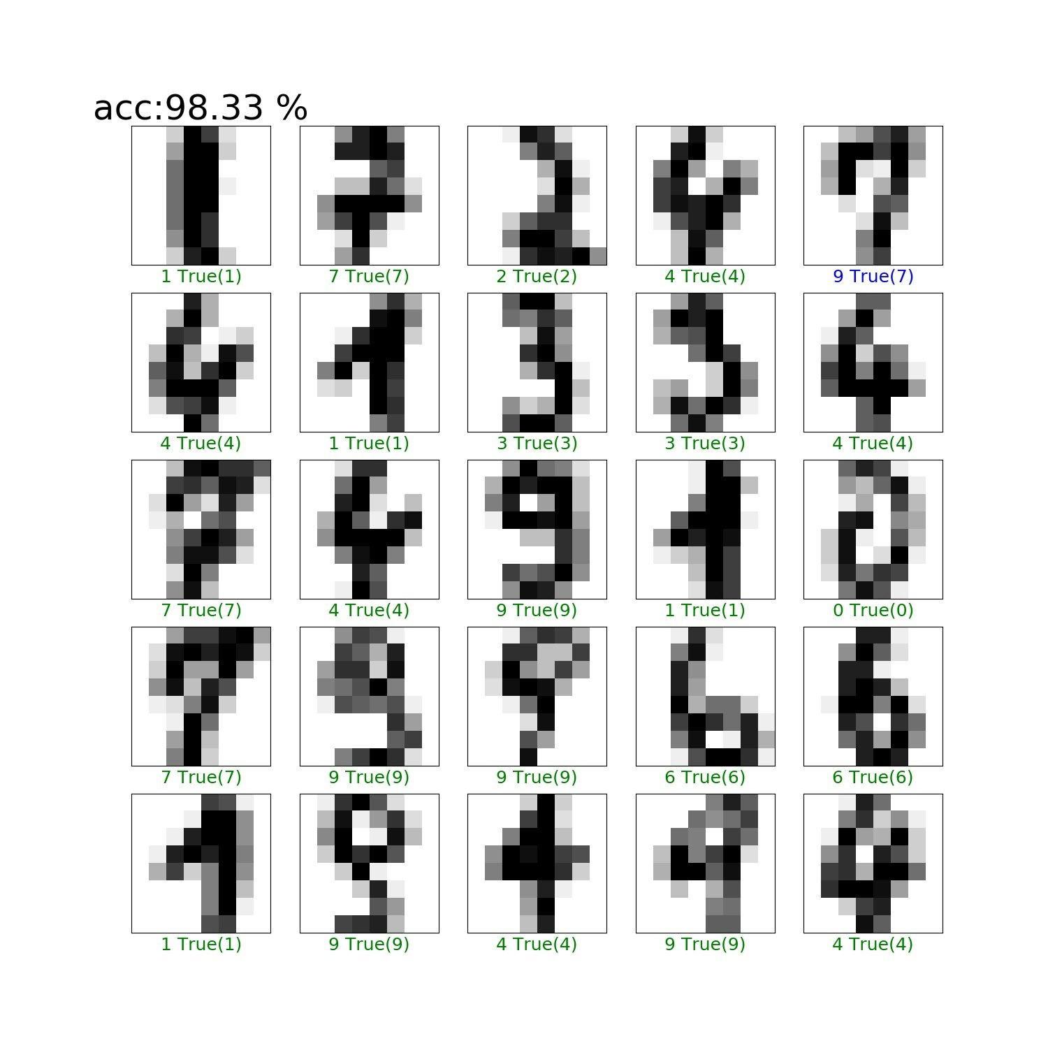
実行結果は以下のとおりで、ランダムフォレストの結果を超えています。
>python RFC.py
acc:98.33 %
まとめ
・SVMでクラス分類をやってみた
・ランダムフォレストのコードにclsの入れ替えだけで手書き文字のクラス分類動いた
・K-means、ランダムフォレスト、そしてSVMだとSVMが一番精度よさそうである
※理由はおまけの追記を確認してください
・【追記】それぞれの理論(K-means、K-近傍法、ランダムフォレスト、そしてSVM)を簡単に解説しようと思う
・DLと合わせて、自前データを分類して精度問題、データの食わせ方の整理をしたい
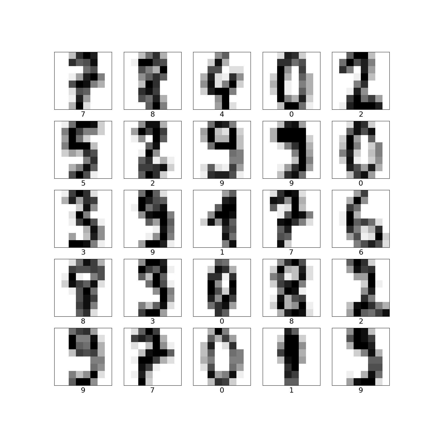
おまけ
from sklearn import datasets
import numpy as np
import matplotlib.pyplot as plt
from sklearn.ensemble import RandomForestClassifier as RFC
from sklearn.model_selection import train_test_split, GridSearchCV
# Import datasets, classifiers and performance metrics
from sklearn import datasets, svm, metrics

mnist = datasets.load_digits()

train_images, test_images, train_labels, test_labels = \
train_test_split(mnist.data, mnist.target, test_size=0.2)

plt.figure(figsize=(15,15))
for i in range(25):
    plt.subplot(5,5,i+1)
    plt.xticks([])
    plt.yticks([])
    plt.imshow(train_images[i].reshape((8,8)), cmap=plt.cm.binary)
    plt.xlabel(train_labels[i], fontsize=18)
plt.savefig('RFC/dataset_input.jpg')
plt.pause(1)
plt.close()
"""
clf = RFC(verbose=True,       # 学習中にログを表示します。この指定はなくてもOK
          n_jobs=-1,          # 複数のCPUコアを使って並列に学習します。-1は最大値。
          random_state=2525)  # 乱数のシードです。
clf.fit(train_images, train_labels)

print(clf.feature_importances_)
"""
# Create a classifier: a support vector classifier
clf = svm.SVC(gamma=0.001)
# We learn the digits on the first half of the digits
clf.fit(train_images, train_labels)

# print(f"acc: {clf.score(test_images, test_labels)}")
acc=clf.score(test_images, test_labels)*100
print("acc:{:.2f} %".format(acc))

predicted_labels = clf.predict(test_images)

plt.figure(figsize=(15,15))
# 先頭から25枚テストデータを可視化
for i in range(25):

    # 画像を作成
    plt.subplot(5,5,i+1)
    plt.xticks([])
    plt.yticks([])
    plt.imshow(test_images[i].reshape((8,8)), cmap=plt.cm.binary)

    # 今プロットを作っている画像データの予測ラベルと正解ラベルをセット
    predicted_label = predicted_labels[i]
    true_label      = test_labels[i]

    # 予測ラベルが正解なら緑、不正解なら赤色を使う
    if predicted_label == true_label:
        color = 'green' # True label color
    else:
        color = 'blue'   # False label color red
    plt.xlabel("{} True({})".format(predicted_label,
                                  true_label), color=color, fontsize=18)
    if i==0:
        plt.title("acc:{:.2f} %".format(acc), fontsize=36)

plt.savefig('RFC/RFC_results.jpg')
plt.pause(1)
plt.close()
【追記】K-近傍法によるirisの分類は、以下のコードを上記のSVMのコードに追記するだけで動きました。なぜか、得られた精度も同じでした。
※冒頭の参考の通り、K-近傍法はK-meansとは異なる手法です
from sklearn.neighbors import KNeighborsClassifier
# from sklearn.cross_validation import train_test_split # trainとtest分割用
# train用とtest用のデータ用意。test_sizeでテスト用データの割合を指定。random_stateはseed値を適当にセット。
# X_train, X_test, Y_train, Y_test = train_test_split(X, Y, test_size = 0.4, random_state=3)

knn = KNeighborsClassifier(n_neighbors=6) # インスタンス生成。n_neighbors:Kの数
knn.fit(X_train, Y_train)                 # モデル作成実行
Y_pred = knn.predict(X_test)              # 予測実行

# 精度確認用のライブラリインポートと実行
# from sklearn import metrics
acc1=metrics.accuracy_score(Y_test, Y_pred)    # 予測精度計測
print("acc1=",acc1)
実行結果は以下のとおり(SVMの結果も併せて表示しています)
※つまり、データ読み込みはSVCのコードのものを利用しており、最後のacc1だけがこのコードの実行結果です
   sepal length (cm)  sepal width (cm)  petal length (cm)  petal width (cm)  \
0                5.1               3.5                1.4               0.2
1                4.9               3.0                1.4               0.2
2                4.7               3.2                1.3               0.2
3                4.6               3.1                1.5               0.2
4                5.0               3.6                1.4               0.2

   target
0  setosa
1  setosa
2  setosa
3  setosa
4  setosa
112 112 38 38
acc= 0.973684210526
acc1= 0.973684210526
【追記】ランダムフォレストのコードにK-近傍法で殴り込みできました
上記のランダムフォレストのコードを以下の部分のみ変更します。
※精度はSVMとほぼ同一の精度になっています
※冒頭の参考の通り、K-近傍法はK-meansとは異なる手法です
"""
clf = RFC(verbose=True,       # 学習中にログを表示します。この指定はなくてもOK
          n_jobs=-1,          # 複数のCPUコアを使って並列に学習します。-1は最大値。
          random_state=2525)  # 乱数のシードです。
clf.fit(train_images, train_labels)

print(clf.feature_importances_)

# Create a classifier: a support vector classifier
clf = svm.SVC(gamma=0.001)
# We learn the digits on the first half of the digits
clf.fit(train_images, train_labels)
"""
from sklearn.neighbors import KNeighborsClassifier
clf = KNeighborsClassifier(n_neighbors=6) # インスタンス生成。n_neighbors:Kの数
clf.fit(train_images, train_labels)
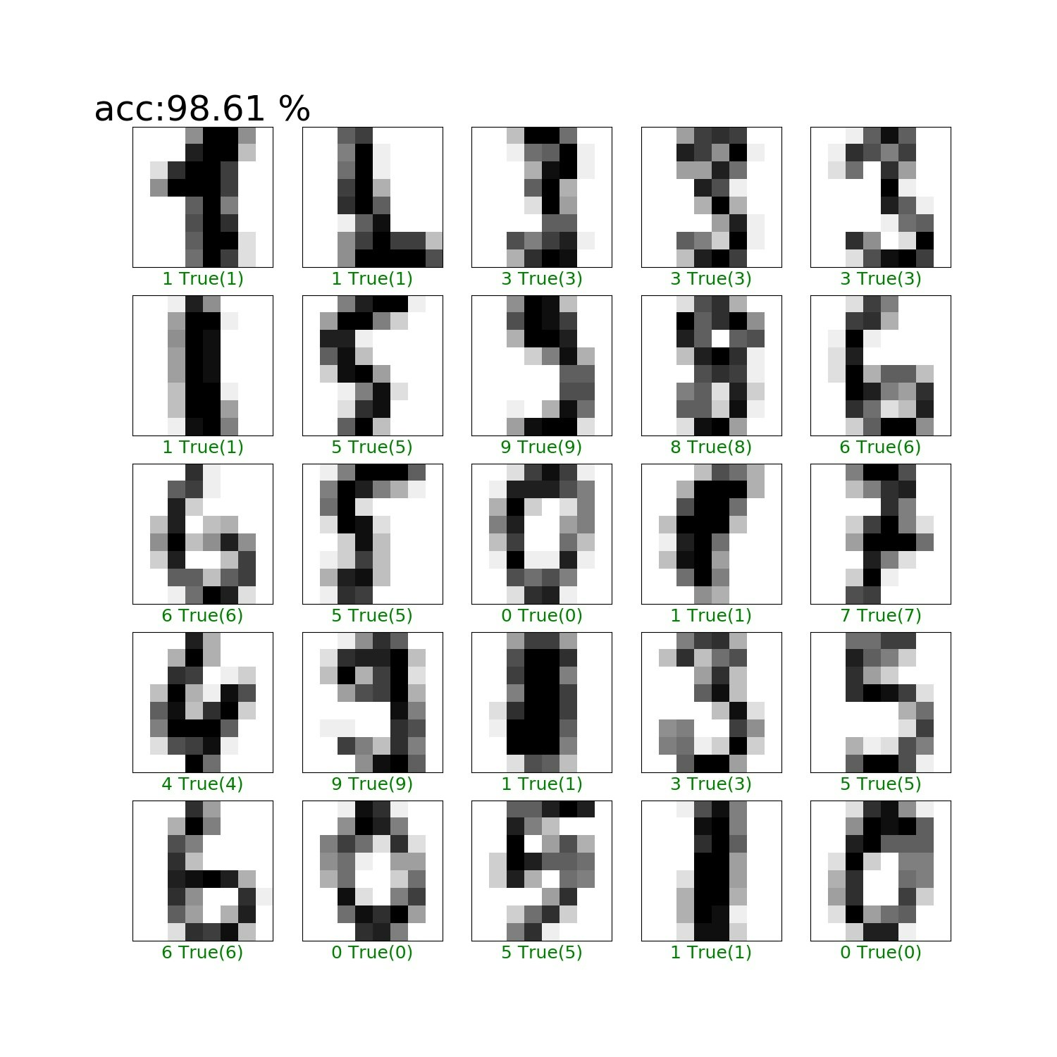
>python RFC.py
acc:98.61 %