【はじめての Databricks】金融取引データから異常検知 #5 リモデル/モデル比較

はじめに

2つ目のモデルを作成、mlflow で1つ目モデルと比較するところまでを行います。

連絡目次

1. 導入/環境設定
2. Collaborative Notebook でデータ可視化
3. Anomaly Detector をデータ探索ツールとして使ってみる
4. 1つ目のモデル構築 (データの偏り 未考慮)
5. [2つ目のモデル構築 (データの偏り 考慮)] (https://qiita.com/Catetin0310/items/0780b4e0f1ba07509930) → 本稿

データセットの分割

1つ目のモデルでは学習に用いるデータセットに偏りがありました。今回はこの課題を解消できるように Train データセットをサンプリングします。

# Train データセットをラベルごとに抽出
dfn = train.filter(train.label == 0)
dfy = train.filter(train.label == 1)

# 要素数
N = train.count()
y = dfy.count()
p = y/N

# 通常取引dfの一部を抜粋、不正取引の df に union
train_b = dfn.sample(False, p, seed = 92285).union(dfy)

# データ全体の要素数、不正取引要素数、構成日比率、train データセットの件数表示
print("Total count: %s \nFraud cases count: %s \nProportion of fraud cases: %s" % (N, y, p))
print("Balanced training dataset count: %s" % train_b.count())

Total count: 5090311
Fraud cases count: 6610
Proportion of fraud cases: 0.0012985454130405784
Balanced training dataset count: 13252

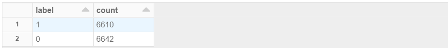
中身を見てみます。通常取引/不正取引でおおよそ半々になっていますね。

display(train_b.groupBy("label").count())

パイプライン修正

バランスが取れたデータセットをモデル学習に利用できるので、今回の評価指標は evaluatorAUC を用います。前記事で作成したパイプラインをそのまま利用します。

# 作成したパイプラインに修正を加えて定義
crossval_b = CrossValidator(estimator = dt,
                          estimatorParamMaps = paramGrid,
                          evaluator = evaluatorAUC,
                          numFolds = 3)  
pipelineCV_b = Pipeline(stages=[indexer, va, crossval_b])

# 新たに作成したデータセットで学習
cvModel_b = pipelineCV_b.fit(train_b)

モデルの作成と分類木の可視化

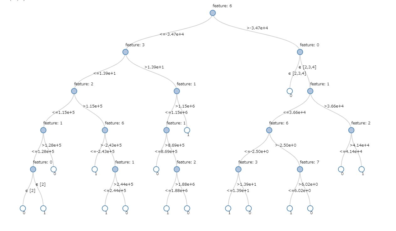
モデルを構築し、樹形図を見てみます。

dt_model_b = pipeline.fit(train_b)
display(dt_model_b.stages[-1])

続いて特徴量の重要度を出力します。

ExtractFeatureImp(dt_model_b.stages[-1].featureImportances, train_pred_b, "features").head(10)

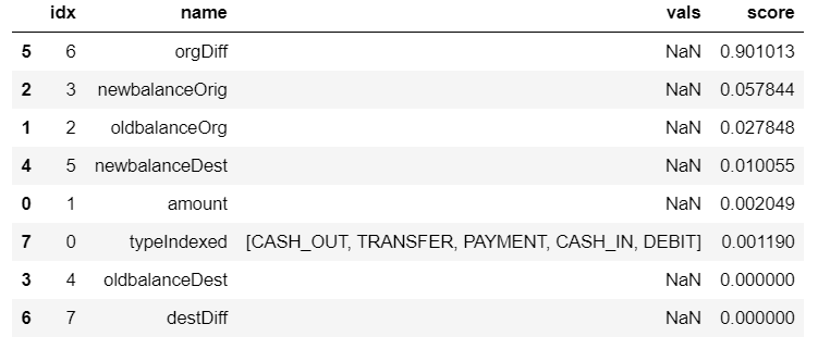
orgDiff (取引実行者の口座残高差分) が重要と判断しているようです。樹形図・利用している特徴量ともに、前回作成したモデルとは全く違いますね。

評価・メトリクスの保存

前回と同様、評価のために必要な情報を導出していきます。

精度指標

# パイプラインの中で一番いいモデルを構築
train_pred_b = cvModel_b.transform(train_b)
test_pred_b = cvModel_b.transform(test)

# Training データで評価指標を算出
pr_train_b = evaluatorPR.evaluate(train_pred_b)
auc_train_b = evaluatorAUC.evaluate(train_pred_b)

# Test データで評価指標算出
pr_test_b = evaluatorPR.evaluate(test_pred_b)
auc_test_b = evaluatorAUC.evaluate(test_pred_b)

# 評価指標の出力
print("PR train:", pr_train_b)
print("AUC train:", auc_train_b)
print("PR test:", pr_test_b)
print("AUC test:", auc_test_b)

PR train: 0.99069584320536
AUC train: 0.9948781444445811
PR test: 0.09312146366332584
AUC test: 0.9929393129548542

混合行列

# 予測結果の一時ビュー作成
test_pred_b.createOrReplaceTempView("test_pred_b")

# テスト結果の混合行列 spark df の作成
test_pred_b_cmdf = spark.sql("select a.label, a.prediction, coalesce(b.count, 0) as count from cmt a left outer join (select label, prediction, count(1) as count from test_pred_b group by label, prediction) b on b.label = a.label and b.prediction = a.prediction order by a.label desc, a.prediction desc")

# Pandas df に変換
cm_b_pdf = test_pred_b_cmdf.toPandas()

# 混合行列の配列生成
cm_b_1d = cm_b_pdf.iloc[:, 2]
TP, FN, FP, TN = cm_b_1d

# 2次元にする
cm_b = np.array([[TP, FN], [FP, TN]])

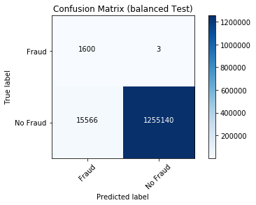
# 混合行列描画 
plot_confusion_matrix(cm_b, "Confusion Matrix (balanced Test)")

メトリクス保存

with mlflow.start_run(experiment_id = mlflow_experiment_id) as run:

  mlflow.log_param("balanced", "yes")
  mlflow.log_metric("AUC train", auc_train_b)
  mlflow.log_metric("AUC test", auc_test_b)
  mlflow.log_metric("PR train", pr_train_b)
  mlflow.log_metric("PR test", pr_test_b)
    
  # モデルのロギング
  mlflow.spark.log_model(dt_model_b, "model")
  
  # 混合行列もログとして残す
  mlflow.log_artifact("confusion-matrix.png")

これで一通りの処理が完了しました。

モデルの比較

前回のモデルと今回のモデルを比較していきます。
数種の評価指標であれば以下のように Notebook で出力・比較可能ですが、この方法では複数のモデルを比較しづらいです。

print("---model #1---")
print("PR train:", pr_train)
print("AUC train:", auc_train)
print("PR test:", pr_test)
print("AUC test:", auc_test)

print("---model #2---")
print("PR train:", pr_train_b)
print("AUC train:", auc_train_b)
print("PR test:", pr_test_b)
print("AUC test:", auc_test_b)

---model #1---
PR train: 0.847168047612724
AUC train: 0.8648916320839469
PR test: 0.8432895226140703
AUC test: 0.8633701428270321

---model #2---
PR train: 0.99069584320536
AUC train: 0.9948781444445811
PR test: 0.09312146366332584
AUC test: 0.9929393129548542

mlflow で比較

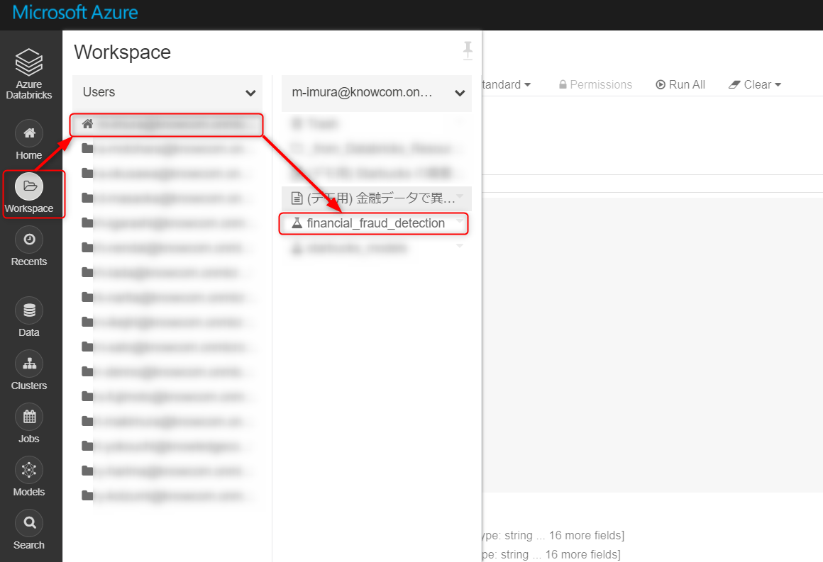
mlflow を用いると比較が容易です。workspace > users と進み、フラスコのアイコンをクリック。

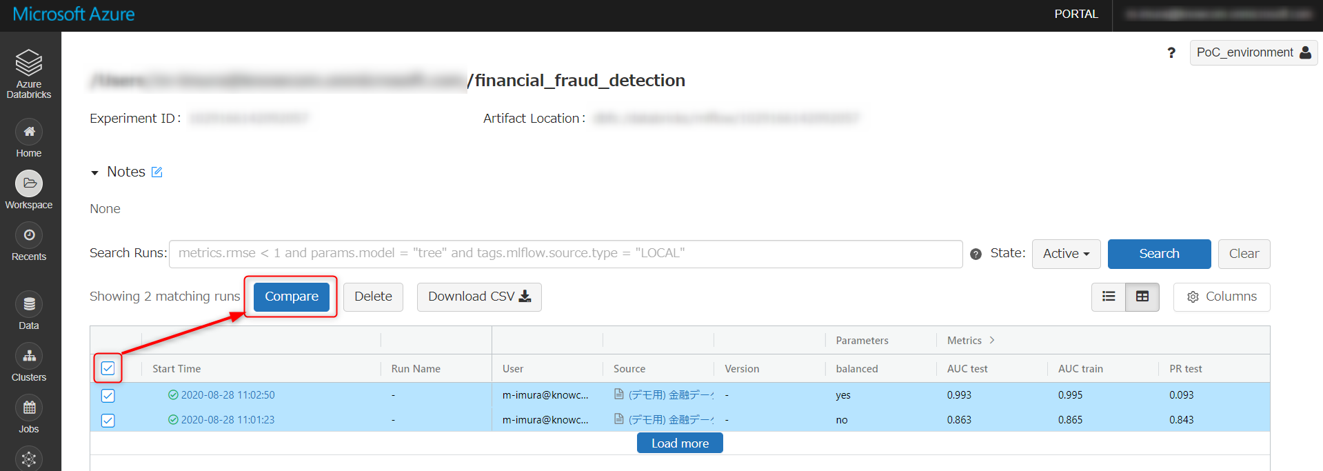
こちらの画面に遷移します。モデルを選択し、Compare をクリック。

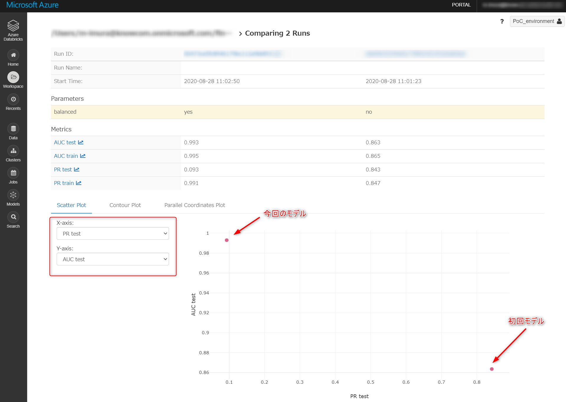
X軸とY軸にそれぞれ PR Test と AUC Test を設定、散布図で比較します。

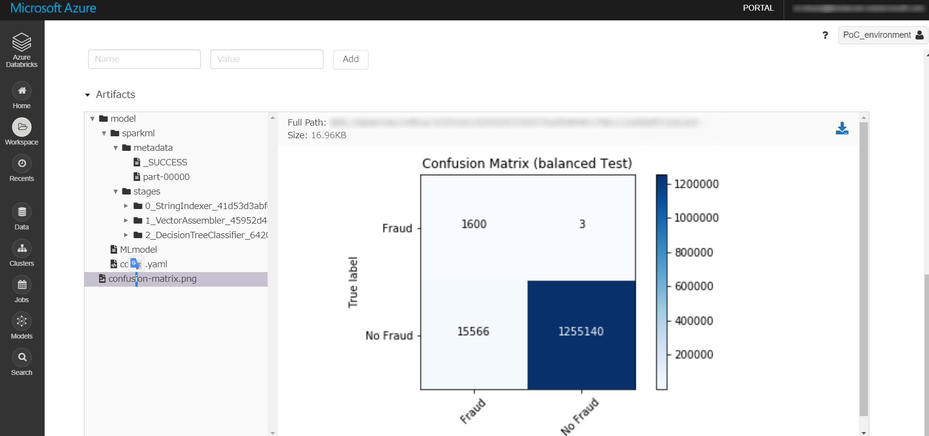
各モデルの ID をクリックすると、モデルそのものや、パイプラインの実行パラメータ、保存しておいた図などにアクセス可能。試行錯誤していると情報が散逸しがちなのでとても便利です。

今回のモデルは「疑わしきはすべて罰する」ようなロジックです。実際に不正検知をはじくフローに組み込むのであれば初回モデルが、当初の要件に沿うためには今回のモデルが合うかもしれません。(いずれも改良必須ですが)

まとめ

5回にわたって金融取引データを可視化、考察、モデル構築、リモデル、比較するところまでをご紹介しました。

本番環境では Azure Datafactory などのデータ関連サービス群を組み入れ、よりシンプルかつ柔軟性の高いアーキテクチャを設計すべきですが、アドホックに機械学習プロジェクトを始めたいという方は、まず Databricks を動かしながらデータ分析の流れを掴んでみてはいかがでしょうか？

参考リンク

datarbicks Resources (公式参考記事集)
Detecting Financial Fraud at Scale with Decision Trees and MLflow on Databricks
mlflow - track machine learning training runs
Synthetic Financial Datasets For Fraud Detection
Binary Classifier Evaluation made easy with HandySpark
notebook