機械学習の必要性が話題になる昨今(2025年11月30日現在)、私もその流れに乗るべく(もとい乗らざるを得なくなったとも言う)機械学習ができる環境を用意することにした。そうはいっても自前のPCで出来るわけもないのでGoogleの力に頼ることにする。
Google Colaboratoryとは
ざっくりいうと、Googleが用意している機械学習用の環境。Googleアカウントひとつで機械学習のためのリソースを拝借してCPU演算からGPU演算、またTPU演算なども行えたりする。
使用言語は主にPython3であり、ほかにもRやJuliaが使用可能。Colaboratoryの環境はJupyter Notebookに近いため、コードを打ち込む個所(コードセル)とテキストを打ち込む箇所(テキストセル)がある種独立している。区分としては対話型の環境らしい。また、次のコマンドでシェルコマンドも実行可能である。
!{Command}
シェルのバージョンは次の通り。
!sh --version
!bash --version

Google Colaboratory上の使用できる機械学習フレームワーク群は次の通り
import tensorflow as tf
import torch
import sklearn
import jax

print("TensorFlow:", tf.__version__)
print(tf.sysconfig.get_build_info())
#
print("PyTorch:", torch.__version__)
print("CUDA available:", torch.cuda.is_available())
print("CUDA version:", torch.version.cuda)
#
print("scikit-learn:", sklearn.__version__)
print("JAX:", jax.__version__)
#
!pip list | grep "torch\|tensorflow\|jax\|sklearn"
実行結果
TensorFlow: 2.19.0
OrderedDict({'cpu_compiler': '/usr/lib/llvm-18/bin/clang', 'cuda_compute_capabilities': ['sm_60', 'sm_70', 'sm_80', 'sm_89', 'compute_90'], 'cuda_version': '12.5.1', 'cudnn_version': '9', 'is_cuda_build': True, 'is_rocm_build': False, 'is_tensorrt_build': False})
PyTorch: 2.9.0+cu126
CUDA available: False
CUDA version: 12.6
scikit-learn: 1.6.1
JAX: 0.7.2
jax                                      0.7.2
jax-cuda12-pjrt                          0.7.2
jax-cuda12-plugin                        0.7.2
jaxlib                                   0.7.2
sklearn-pandas                           2.2.0
tensorflow                               2.19.0
tensorflow-datasets                      4.9.9
tensorflow_decision_forests              1.12.0
tensorflow-hub                           0.16.1
tensorflow-metadata                      1.17.2
tensorflow-probability                   0.25.0
tensorflow-text                          2.19.0
torch                                    2.9.0+cu126
torchao                                  0.10.0
torchaudio                               2.9.0+cu126
torchdata                                0.11.0
torchsummary                             1.5.1
torchtune                                0.6.1
torchvision                              0.24.0+cu126
その他の詳しい使い方はこちらから
Google Colaboratory よくある質問
機械学習をやってみる
とりあえずChatGPT様にサンプルコードを作ってもらい、そのコードでやってみた。
Google Colaboratoryでの使用を前提としているので注意。
※コードが思いのほか長かったので折りたたんでいます。
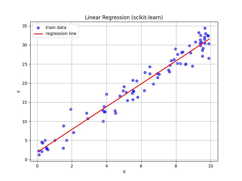
scikit-learn:線形回帰
コードと実行結果
# Google Driveと接続してデータのやりとりをするためのライブラリ
from google.colab import drive

# 機械学習用のライブラリ
from sklearn.linear_model import LinearRegression
from sklearn.model_selection import train_test_split
from sklearn.metrics import mean_squared_error
import numpy as np
import matplotlib.pyplot as plt

# Google Driveとのマウント
drive.mount('/content/drive/')

# ------------------------
# データ生成
# ------------------------
# ダミーデータ( y = 3x + 2 + ノイズ )
X = np.random.rand(100, 1) * 10
y = 3 * X + 2 + np.random.randn(100, 1) * 2

# データ分割
X_train, X_test, y_train, y_test = train_test_split(X, y, test_size=0.2)

# ------------------------
# モデル学習
# ------------------------
model = LinearRegression()
model.fit(X_train, y_train)

# 予測
y_pred = model.predict(X_test)

# 結果表示
print("回帰係数:", model.coef_)
print("切片:", model.intercept_)
print("MSE:", mean_squared_error(y_test, y_pred))

# ------------------------
# 可視化(散布図+回帰直線)
# ------------------------
plt.figure(figsize=(8, 6))

# 学習データの散布図
plt.scatter(X_train, y_train, color='blue', label="train data", alpha=0.6)

# 学習した回帰直線を描画
x_line = np.linspace(X.min(), X.max(), 100).reshape(-1, 1)
y_line = model.predict(x_line)
plt.plot(x_line, y_line, color='red', label="regression line", linewidth=2)

plt.xlabel("X")
plt.ylabel("y")
plt.title("Linear Regression (scikit-learn)")
plt.legend()
plt.grid(True)
plt.savefig('/content/drive/ *保存したいディレクトリとファイル名* ')
plt.show()
実行結果
TensorFlow/Keras:MNIST
コードと実行結果
# Google Driveと接続してデータのやりとりをするためのライブラリ
from google.colab import drive
#
import tensorflow as tf
from tensorflow.keras import layers, models
import matplotlib.pyplot as plt
import numpy as np
from sklearn.metrics import confusion_matrix, ConfusionMatrixDisplay
# Google Driveとのマウント
drive.mount('/content/drive/')
# ------------------------
# データロード
# ------------------------
(x_train, y_train), (x_test, y_test) = tf.keras.datasets.mnist.load_data()
# 正規化&reshape
x_train = x_train.reshape(-1, 28*28).astype("float32") / 255
x_test = x_test.reshape(-1, 28*28).astype("float32") / 255
# ------------------------
# モデル構築
# ------------------------
model = models.Sequential([
layers.Dense(128, activation="relu"),
layers.Dense(10, activation="softmax")
])
# コンパイル
model.compile(optimizer="adam",
loss="sparse_categorical_crossentropy",
metrics=["accuracy"])
# ------------------------
# 学習
# ------------------------
history = model.fit(
x_train, y_train,
epochs=3,
batch_size=32,
validation_split=0.1,
verbose=1
)
# ------------------------
# 評価
# ------------------------
test_loss, test_acc = model.evaluate(x_test, y_test, verbose=0)
print("テスト精度:", test_acc)
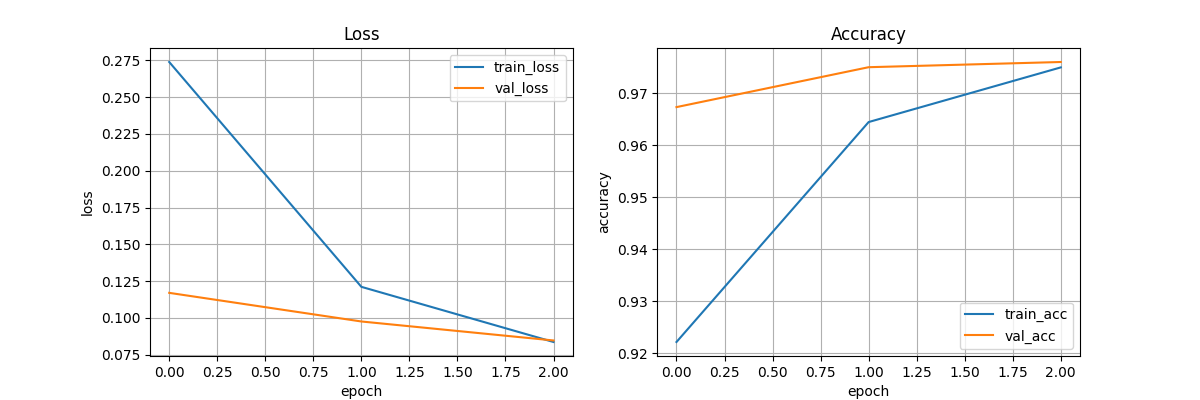
# ============================================================
# ① 学習曲線(Loss / Accuracy)
# ============================================================
plt.figure(figsize=(12, 4))
# Loss
plt.subplot(1, 2, 1)
plt.plot(history.history["loss"], label="train_loss")
plt.plot(history.history["val_loss"], label="val_loss")
plt.title("Loss")
plt.xlabel("epoch")
plt.ylabel("loss")
plt.legend()
plt.grid(True)
# Accuracy
plt.subplot(1, 2, 2)
plt.plot(history.history["accuracy"], label="train_acc")
plt.plot(history.history["val_accuracy"], label="val_acc")
plt.title("Accuracy")
plt.xlabel("epoch")
plt.ylabel("accuracy")
plt.legend()
plt.grid(True)
plt.savefig("/content/drive/ *保存したいディレクトリとファイル名* ")
plt.show()
# ============================================================
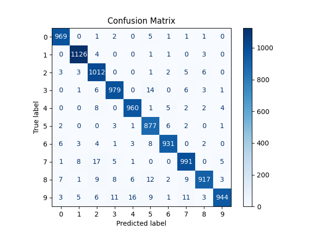
# ② 混同行列(Confusion Matrix)
# ============================================================
# 予測
y_pred = np.argmax(model.predict(x_test), axis=1)
cm = confusion_matrix(y_test, y_pred)
disp = ConfusionMatrixDisplay(confusion_matrix=cm)
plt.figure(figsize=(8, 8))
disp.plot(cmap="Blues", values_format="d")
plt.title("Confusion Matrix")
plt.savefig("/content/drive/ *保存したいディレクトリとファイル名* ")
plt.show()
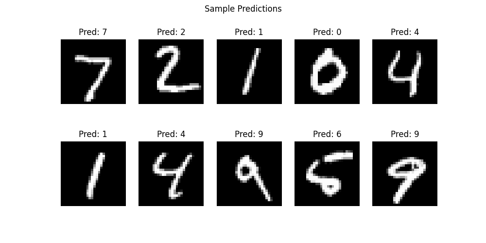
# ============================================================
# ③ 予測結果の可視化(例をいくつか)
# ============================================================
plt.figure(figsize=(10, 5))
for i in range(10):
plt.subplot(2, 5, i+1)
img = x_test[i].reshape(28, 28)
plt.imshow(img, cmap="gray")
plt.title(f"Pred: {y_pred[i]}")
plt.axis("off")
plt.suptitle("Sample Predictions")
plt.savefig("/content/drive/ *保存したいディレクトリとファイル名* ")
plt.show()
実行結果
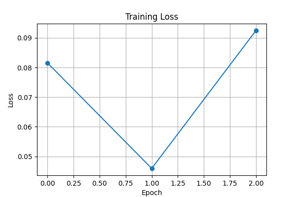
PyTorch:MNIST
コードと実行結果
# Google Driveと接続してデータのやりとりをするためのライブラリ
from google.colab import drive
#
import torch
import torch.nn as nn
import torch.optim as optim
from torchvision import datasets, transforms
from torch.utils.data import DataLoader
import matplotlib.pyplot as plt
from sklearn.metrics import confusion_matrix, ConfusionMatrixDisplay
import numpy as np

# Google Driveとのマウント
drive.mount('/content/drive/')

# ------------------------
# データセット準備
# ------------------------
transform = transforms.Compose([transforms.ToTensor()])

train_dataset = datasets.MNIST(root="./data", train=True, download=True, transform=transform)
test_dataset  = datasets.MNIST(root="./data", train=False, transform=transform)

train_loader = DataLoader(train_dataset, batch_size=64, shuffle=True)
test_loader  = DataLoader(test_dataset, batch_size=1000, shuffle=False)

# ------------------------
# モデル定義
# ------------------------
class Net(nn.Module):
    def __init__(self):
        super().__init__()
        self.fc1 = nn.Linear(28*28, 128)
        self.fc2 = nn.Linear(128, 10)

    def forward(self, x):
        x = x.view(-1, 28*28)
        x = torch.relu(self.fc1(x))
        x = self.fc2(x)
        return x

model = Net()

# ------------------------
# 損失関数・最適化
# ------------------------
criterion = nn.CrossEntropyLoss()
optimizer = optim.Adam(model.parameters())

# ------------------------
# 学習ループ
# ------------------------
num_epochs = 3
train_losses = []

for epoch in range(num_epochs):
    model.train()
    for data, target in train_loader:
        optimizer.zero_grad()
        output = model(data)
        loss = criterion(output, target)
        loss.backward()
        optimizer.step()

    train_losses.append(loss.item())
    print(f"Epoch {epoch+1}/{num_epochs}, Loss: {loss.item()}")

print("学習完了!")

# ------------------------
# テスト精度
# ------------------------
model.eval()
correct = 0
total = 0
pred_list = []
true_list = []

with torch.no_grad():
    for data, target in test_loader:
        output = model(data)
        pred = output.argmax(dim=1)
        correct += (pred == target).sum().item()
        total += target.size(0)

        pred_list.extend(pred.numpy())
        true_list.extend(target.numpy())

test_acc = correct / total
print("テスト精度:", test_acc)

# ============================================================
# ① 学習曲線(Loss)
# ============================================================
plt.figure(figsize=(6, 4))
plt.plot(train_losses, marker="o")
plt.title("Training Loss")
plt.xlabel("Epoch")
plt.ylabel("Loss")
plt.grid(True)
plt.savefig("/content/drive/ *保存したいディレクトリとファイル名* ")
plt.show()

# ============================================================
# ② 混同行列(Confusion Matrix)
# ============================================================
cm = confusion_matrix(true_list, pred_list)

plt.figure(figsize=(8, 8))
disp = ConfusionMatrixDisplay(confusion_matrix=cm)
disp.plot(cmap="Blues", values_format="d")
plt.title("Confusion Matrix")
plt.savefig("/content/drive/ *保存したいディレクトリとファイル名* ")
plt.show()

# ============================================================
# ③ 予測画像の可視化(10 個)
# ============================================================
plt.figure(figsize=(10, 5))
for i in range(10):
    img, label = test_dataset[i]
    pred = model(img.unsqueeze(0)).argmax(dim=1).item()

    plt.subplot(2, 5, i+1)
    plt.imshow(img.squeeze(), cmap="gray")
    plt.title(f"Label:{label}, Pred:{pred}")
    plt.axis("off")

plt.suptitle("Sample Predictions")
plt.savefig("/content/drive/ *保存したいディレクトリとファイル名* ")
plt.show()
実行結果


締め
Googleアカウントだけで使用できるリソースは限られているものの(選べるハードウェアが少なかったり利用時間に制限があったり)、まず触ってみるというときには非常にありがたい環境といえるだろう。
主に使用される機械学習フレームワークはインストール済で、簡単に利用できるのも心強い。
最後に
Chat GPT様は偉大であらせられる。