0. はじめに
今回は学習モデルの手法の一つである、LightGBM について調べてみました。
LightGBM はアンサンブル学習のひとつとして Kaggle でもよく利用されます。
伴って、その周辺のプロセス(ROC曲線のプロットなど)も必要になるので、ついでにまとめておきました。
参考にした記事はこちらです。
1. LightGBM のインストール
pip install lightgbm
します。しかし、
import lightgbm as lgb
でエラーが出たので対処法を調べたところ、
に辿り着きました。
これに従って、
brew install libomp
をすると、無事解決しました。
これで先に進めます。
2. 擬似的なデータセットを用意する
まずは必要なライブラリをインポートします。
%matplotlib inline
import numpy as np
import pandas as pd
import matplotlib.pyplot as plt

print(pd.__version__) #スクリプト上でバージョンを確認できる。
0.21.0
次にデータセットを読み込みます。
今回は scikit-learn のデータセットにあるアヤメのデータを使用します。
from sklearn.datasets import load_iris

iris = load_iris()
# print(iris.DESCR)  #データセットに関する説明を表示
print(type(iris))
<class 'sklearn.utils.Bunch'>
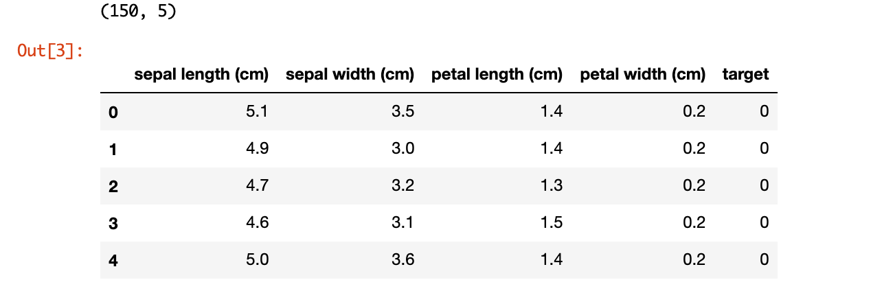
df = pd.DataFrame(iris.data, columns=iris.feature_names)
df['target'] = iris.target

print(df.shape)
df.head()
2変数だけでこのデータをプロットしてみます。
fig = plt.figure(figsize = (5,5))
ax = fig.add_subplot(111)

plt.scatter(df[df['target']==0].iloc[:,0], df[df['target']==0].iloc[:,1], label='Setosa')
plt.scatter(df[df['target']==1].iloc[:,0], df[df['target']==1].iloc[:,1], label='Versicolour')
plt.scatter(df[df['target']==2].iloc[:,0], df[df['target']==2].iloc[:,1], label='Virginica')
plt.xlabel("sepal length[cm]", fontsize=13)
plt.ylabel("sepal width[cm]", fontsize=13)

plt.legend()
plt.show()
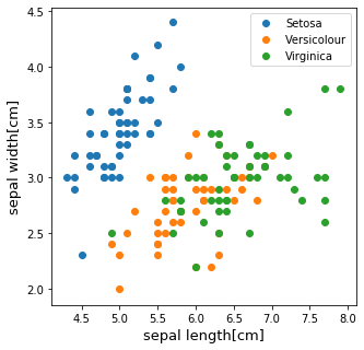
今回はこの3種類の中で比較的に分類が難しそうな Versicolour と Virginica の2クラス分類問題として解いてみようと思います。そのため、ラベルが0のものは除外し。残りの2種類に0と1のラベルを与えます。
data = df[df['target']!=0]
data.head()
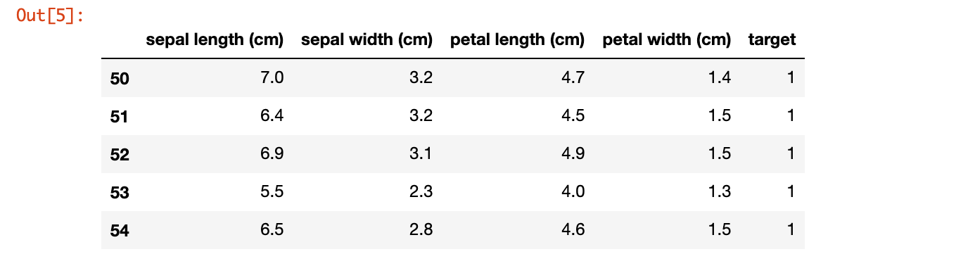
data['target'] = data['target'] - 1

X = data.drop('target', axis=1)
y = data['target']
/Users/{user}/.pyenv/versions/3.6.6/lib/python3.6/site-packages/ipykernel_launcher.py:1: SettingWithCopyWarning:
A value is trying to be set on a copy of a slice from a DataFrame.
Try using .loc[row_indexer,col_indexer] = value instead

See the caveats in the documentation: http://pandas.pydata.org/pandas-docs/stable/indexing.html#indexing-view-versus-copy
  """Entry point for launching an IPython kernel.
このWarningをうまく処理できなかったので、対処法をご存知の方は教えてください...
3. LightGBMで学習する
その前に、訓練データとテストデータを分割します。今回は、交叉検証を行うので validation データも用意して置きます。
from sklearn.model_selection import train_test_split

X_trainval, X_test, y_trainval, y_test = train_test_split(X, y, test_size=0.2, random_state=7, stratify=y)
X_train, X_val, y_train, y_val = train_test_split(X_trainval, y_trainval, test_size=0.2, random_state=7, stratify=y_trainval)
ようやく本題です。lightgbm モデルを構築していきます。
ハイパーパラメーターについて
lightgbmの関数trainの引数paramsやその他の引数がハイパーパラメーターになります。
それに関するドキュメンテーションはこちらです。
また、以下の記事も参考になると思います。
ここでは、重要そうなものだけ説明しておきます。
- objective : 今回は2クラス分類なので binary を指定しています。
- metric : 2クラス分類に使用可能な指標のひとつである auc を指定しています。
- early_stopping_rounds : 指定したラウンド数で metric が改善しない場合、その前で学習を打ち切る。
※理解が誤っているかもしれませんが、その時は訂正お願いします。
import lightgbm as lgb

lgb_train = lgb.Dataset(X_train, y_train)
lgb_val = lgb.Dataset(X_val, y_val)

params = {
    'metric' :'auc', #binary_logloss でも可能
    'objective' :'binary',
    'max_depth' :1,
    'num_leaves' :2,
    'min_data_in_leaf' : 5,
}

evals_result = {} #結果を格納するための辞書

gbm = lgb.train(params,
                lgb_train,
                valid_sets = [lgb_train, lgb_val],
                valid_names = [ 'train', 'eval'],
                num_boost_round = 500,
                early_stopping_rounds = 20,
                verbose_eval = 10,
                evals_result = evals_result
               )
Training until validation scores don't improve for 20 rounds
[10]	train's auc: 0.997559	eval's auc: 0.914062
[20]	train's auc: 0.997559	eval's auc: 0.914062
Early stopping, best iteration is:
[3]	train's auc: 0.998047	eval's auc: 0.914062
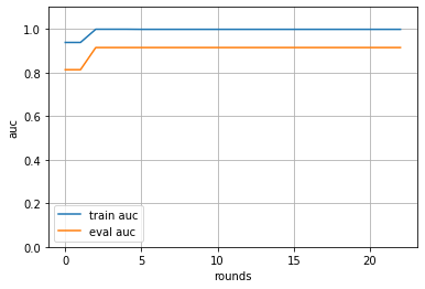
4. 学習曲線をプロットする
先ほどの train 関数の引数に入れておいた evals_result の中に指標に指定しておいた auc に関する記録が含まれています。
これを利用して学習曲線を書いていきます。
print(evals_result.keys())
print(evals_result['eval'].keys())
print(evals_result['train'].keys())

train_metric = evals_result['train']['auc']
eval_metric = evals_result['eval']['auc']
train_metric[:5], eval_metric[:5]
dict_keys(['train', 'eval'])
odict_keys(['auc'])
odict_keys(['auc'])

([0.9375, 0.9375, 0.998046875, 0.998046875, 0.998046875],
 [0.8125, 0.8125, 0.9140625, 0.9140625, 0.9140625])
このように辞書の中にリストとして含まれているので、キーを指定してこのリストを取得します。
そして、学習曲線を描きます。
plt.plot(train_metric, label='train auc')
plt.plot(eval_metric, label='eval auc')
plt.grid()
plt.legend()
plt.ylim(0, 1.1)

plt.xlabel('rounds')
plt.ylabel('auc')
plt.show()
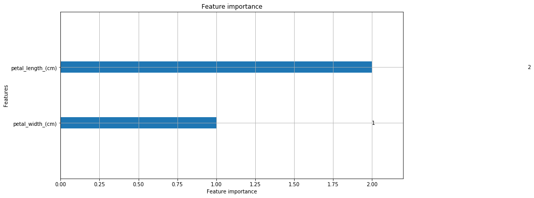
5. 重要な特徴量を調べる
lightgbm は分類の際の重要度を lightgbm.plot_importance を使って可視化することができます。
lightgbm.plot_importance のドキュメンテーションはこちらです。
lgb.plot_importance(gbm, figsize=(12, 6), max_num_features=4)
plt.show();
6. テストデータを推定する・ROC曲線をプロットする
from sklearn import metrics

y_pred = gbm.predict(X_test, num_iteration=gbm.best_iteration)

fpr, tpr, thresholds = metrics.roc_curve(y_test, y_pred, drop_intermediate=False, )
auc = metrics.auc(fpr, tpr)
print('auc:', auc)
auc: 1.0
roc_curve のドキュメンテーションはこちらです。
またROC曲線について調べていた際に、以下の記事が分かりやすくまとまっていたのでリンクしておきます。
plt.plot(fpr, tpr, marker='o')
plt.xlabel('FPR: False positive rate')
plt.ylabel('TPR: True positive rate')
plt.grid()
plt.plot();

今回は比較的簡単なものだったので、極端なROC曲線になりました。
最後に、ある閾値を設定し、その閾値を基準に回答ラベルを振り分けます。
y_pred = (y_pred >= 0.5).astype(int)
y_pred
array([1, 0, 1, 1, 0, 1, 0, 0, 0, 1, 1, 1, 0, 0, 0, 1, 0, 0, 1, 0])
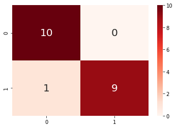
7. 混同行列のヒートマップを描く
最後に、
を参考にして、混同行列のヒートマップも描いてみました。
from sklearn.metrics import confusion_matrix
import seaborn as sns
import matplotlib.pyplot as plt

cm = confusion_matrix(y_test.values, y_pred)

sns.heatmap(cm, annot=True, annot_kws={'size': 20}, cmap= 'Reds');