『機械学習のエッセンス(http://isbn.sbcr.jp/93965/)』のPythonサンプルをJuliaで書き換えてみる。（第04章08数理最適化）

はじめに

『機械学習のエッセンス(http://isbn.sbcr.jp/93965/)』のPythonサンプルをJuliaで書き換えてみる。（第04章07データの可視化）の続きです。

Juliaのバージョン

2019-01-21にJuliaのバージョン1.1がリリースされました。
https://github.com/JuliaLang/julia/blob/v1.1.0/NEWS.md

いままで1.0.3でサンプルを作成していましたが、1.1にアップグレードしました。

               _
   _       _ _(_)_     |  Documentation: https://docs.julialang.org
  (_)     | (_) (_)    |
   _ _   _| |_  __ _   |  Type "?" for help, "]?" for Pkg help.
  | | | | | | |/ _` |  |
  | | |_| | | | (_| |  |  Version 1.1.0 (2019-01-21)
 _/ |\__'_|_|_|\__'_|  |  Official https://julialang.org/ release
|__/                   |

準備

参考にしたサイトは最後に載せました。

Plotsパッケージインストール

• 後で使うPlotsパッケージはJuliaのバージョン1.0.3でインストール済だったのですが、1.1にアップグレードした後インストールをし直す必要がありました。

未インストールの場合、JuliaのREPLで下記のコマンドを実行します。

julia> using Pkg

julia> Pkg.add("Plots")

数理最適化パッケージのインストール

• Jump：最適化モデリングツール
• Clp：線形計画法のソルバー
• OSQP：2次計画法のソルバー

JuliaのREPLで下記のコマンドを実行します。

julia> using Pkg

julia> Pkg.add("JuMP")
（出力略）
julia> Pkg.add("Clp")
（出力略）
julia> Pkg.add("OSQP")
（出力略）

線形計画問題

\begin{alignat}{2}
\text{Maximize} &\quad  3x + 4y \\
\text{Subject to} &\quad  x + 4y \le 1700 \\
                  &\quad 2x + 3y \le 1400 \\
                 &\quad 2x + y \le 1000 \\
                 &\quad x \ge 0 \\
                 &\quad y \ge 0 \\
\end{alignat}

本のPythonサンプルでは関数の仕様に合わせて目的関数の最小化にしていますが、Juliaのライブラリではそのまま最大化（Max)で指定できるようなのでそれで書きました。
参考にしたサイトでは@を多用した書き方になっていました。Juliaはマクロというものが使えるとのことで、使いこなせると便利そうです。
https://docs.julialang.org/en/v1/manual/metaprogramming/index.html

lp1.jl

using JuMP
using Clp

m = Model(solver=ClpSolver())
@variable(m, x >= 0)
@variable(m, y >= 0)

@objective(m, Max, 3 * x + 4 * y )

@constraint(m, x + 4 * y <= 1700)
@constraint(m, 2 * x + 3 * y <= 1400)
@constraint(m, 2 * x + y <= 1000)

status = solve(m)

println(getvalue(x))
println(getvalue(y))
println(getobjectivevalue(m))

実行結果

julia> include("lp1.jl")
399.99999999999994
200.0
1999.9999999999998

それぞれ上から、$x$,$y$,最適値です。本だと400,200,-2000（最小値）となっているので、微妙に誤差が出ています。

Minで書き直す

本と同じように目的関数の最小化で書いてみます。

@objective(m, Max, 3 * x + 4 * y )
の部分を
@objective(m, Min, (-3) * x + (-4) * y )
に変更しました。

lp1-min.jl

using JuMP
using Clp

m = Model(solver=ClpSolver())
@variable(m, x >= 0)
@variable(m, y >= 0)

@objective(m, Min, (-3) * x + (-4) * y )

@constraint(m, x + 4 * y <= 1700)
@constraint(m, 2 * x + 3 * y <= 1400)
@constraint(m, 2 * x + y <= 1000)

status = solve(m)

println(getvalue(x))
println(getvalue(y))
println(getobjectivevalue(m))

実行結果

julia> include("lp1-min.jl")
399.99999999999994
200.0
-1999.9999999999998

2次計画法

f(x, y) = x^2 + xy + y^2 + 2x + 4y

ベクトルによる記述

本のPythonサンプルと同じ方法です。

qp1.jl

using JuMP
using OSQP

solver = OSQPMathProgBaseInterface.OSQPSolver()
m = Model(solver=solver)

@variable(m, x[1:2])

P = [2 1
     1 2]
q = [2, 4]
@objective(m, Min, 0.5 * x'*P*x + q'*x)

status = solve(m)

println(getvalue(x))
println(getobjectivevalue(m))

実行結果

julia> include("qp1.jl")
-----------------------------------------------------------------
           OSQP v0.5.0  -  Operator Splitting QP Solver
              (c) Bartolomeo Stellato,  Goran Banjac
        University of Oxford  -  Stanford University 2018
-----------------------------------------------------------------
problem:  variables n = 2, constraints m = 2
          nnz(P) + nnz(A) = 5
settings: linear system solver = qdldl,
          eps_abs = 1.0e-03, eps_rel = 1.0e-03,
          eps_prim_inf = 1.0e-04, eps_dual_inf = 1.0e-04,
          rho = 1.00e-01 (adaptive),
          sigma = 1.00e-06, alpha = 1.60, max_iter = 4000
          check_termination: on (interval 25),
          scaling: on, scaled_termination: off
          warm start: on, polish: off

iter   objective    pri res    dua res    rho        time
   1  -2.5600e+00   1.42e-21   2.40e+00   1.00e-01   4.03e-05s
  25  -4.0000e+00   3.73e-16   1.14e-05   1.00e-01   5.42e-05s

status:               solved
number of iterations: 25
optimal objective:    -4.0000
run time:             6.12e-05s
optimal rho estimate: 1.00e-06

[-1.20161e-9, -2.00001]
-3.99999999996769

出力が多いですが、最後の2行が結果です。
本と少し誤差がありますが、$(x, y) = (0, -2)$、最適値-4となり、同じ結果が得られました。

スカラー変数での記述

線形計画問題の時と同じように、目的関数をそのまま指定することも出来るようです。

qp1-2.jl

using JuMP
using OSQP

solver = OSQPMathProgBaseInterface.OSQPSolver()
m = Model(solver=solver)

@variable(m, x)
@variable(m, y)

@objective(m, Min, x^2 + x*y + y^2 + 2x + 4y)

status = solve(m)

println(getvalue(x))
println(getvalue(y))
println(getobjectivevalue(m))

実行結果

julia> include("qp1-2.jl")
-----------------------------------------------------------------
           OSQP v0.5.0  -  Operator Splitting QP Solver
              (c) Bartolomeo Stellato,  Goran Banjac
        University of Oxford  -  Stanford University 2018
-----------------------------------------------------------------
problem:  variables n = 2, constraints m = 2
          nnz(P) + nnz(A) = 5
settings: linear system solver = qdldl,
          eps_abs = 1.0e-03, eps_rel = 1.0e-03,
          eps_prim_inf = 1.0e-04, eps_dual_inf = 1.0e-04,
          rho = 1.00e-01 (adaptive),
          sigma = 1.00e-06, alpha = 1.60, max_iter = 4000
          check_termination: on (interval 25),
          scaling: on, scaled_termination: off
          warm start: on, polish: off

iter   objective    pri res    dua res    rho        time
   1  -2.5600e+00   1.42e-21   2.40e+00   1.00e-01   5.08e-05s
  25  -4.0000e+00   3.73e-16   1.14e-05   1.00e-01   7.29e-05s

status:               solved
number of iterations: 25
optimal objective:    -4.0000
run time:             8.43e-05s
optimal rho estimate: 1.00e-06

-1.2016118660344087e-9
-2.0000056836540048
-3.99999999996769

同じく$(x, y) = (0, -2)$、最適値-4が得られました。

制約付きの2次計画問題

式04-08

\begin{alignat}{2}
\text{Minimize} &\quad  f(x, y) = x^2 + xy + y^2 + 2x + 4y \\
\text{Subject to} &\quad  x + y = 0 \\
\end{alignat}

ベクトルによる記述

qp2.jl

using JuMP
using OSQP

solver = OSQPMathProgBaseInterface.OSQPSolver()
m = Model(solver=solver)

@variable(m, x[1:2])

A = [1, 1]
b = 0
@constraint(m, A'*x == b)

P = [2 1
     1 2]
q = [2, 4]
@objective(m, Min, 0.5 * x'*P*x + q'*x)

status = solve(m)

println(getvalue(x))
println(getobjectivevalue(m))

実行結果

julia> include("qp2.jl")
-----------------------------------------------------------------
           OSQP v0.5.0  -  Operator Splitting QP Solver
              (c) Bartolomeo Stellato,  Goran Banjac
        University of Oxford  -  Stanford University 2018
-----------------------------------------------------------------
problem:  variables n = 2, constraints m = 3
          nnz(P) + nnz(A) = 7
settings: linear system solver = qdldl,
          eps_abs = 1.0e-03, eps_rel = 1.0e-03,
          eps_prim_inf = 1.0e-04, eps_dual_inf = 1.0e-04,
          rho = 1.00e-01 (adaptive),
          sigma = 1.00e-06, alpha = 1.60, max_iter = 4000
          check_termination: on (interval 25),
          scaling: on, scaled_termination: off
          warm start: on, polish: off

iter   objective    pri res    dua res    rho        time
   1  -6.7012e-01   1.01e-02   2.40e+00   1.00e-01   4.20e-05s
  25  -1.0000e+00   1.08e-06   1.14e-05   1.00e-01   5.73e-05s

status:               solved
number of iterations: 25
optimal objective:    -1.0000
run time:             6.45e-05s
optimal rho estimate: 6.16e-02

[1.0, -1.0]
-1.0000032372275154

$(x,y) = (1, -1)$、最適値-1で、本と同じ結果が得られました。

スカラー変数での記述

qp2-2.jl

using JuMP
using OSQP

solver = OSQPMathProgBaseInterface.OSQPSolver()
m = Model(solver=solver)

@variable(m, x)
@variable(m, y)

@constraint(m, x + y == 0)
@objective(m, Min, x^2 + x*y + y^2 + 2x + 4y)

status = solve(m)

println(getvalue(x))
println(getvalue(y))
println(getobjectivevalue(m))

実行結果

julia> include("qp2-2.jl")
-----------------------------------------------------------------
           OSQP v0.5.0  -  Operator Splitting QP Solver
              (c) Bartolomeo Stellato,  Goran Banjac
        University of Oxford  -  Stanford University 2018
-----------------------------------------------------------------
problem:  variables n = 2, constraints m = 3
          nnz(P) + nnz(A) = 7
settings: linear system solver = qdldl,
          eps_abs = 1.0e-03, eps_rel = 1.0e-03,
          eps_prim_inf = 1.0e-04, eps_dual_inf = 1.0e-04,
          rho = 1.00e-01 (adaptive),
          sigma = 1.00e-06, alpha = 1.60, max_iter = 4000
          check_termination: on (interval 25),
          scaling: on, scaled_termination: off
          warm start: on, polish: off

iter   objective    pri res    dua res    rho        time
   1  -6.7012e-01   1.01e-02   2.40e+00   1.00e-01   4.65e-05s
  25  -1.0000e+00   1.08e-06   1.14e-05   1.00e-01   6.76e-05s

status:               solved
number of iterations: 25
optimal objective:    -1.0000
run time:             7.89e-05s
optimal rho estimate: 6.16e-02

1.0000023016867856
-1.000003380765606
-1.0000032372275154

$(x,y) = (1, -1)$、最適値-1。

式04-09

\begin{alignat}{2}
\text{Minimize} &\quad  f(x, y) = x^2 + xy + y^2 + 2x + 4y \\
\text{Subject to} &\quad  2x + 3y \le 3 \\
\end{alignat}

ベクトルによる記述

qp3.jl

using JuMP
using OSQP

solver = OSQPMathProgBaseInterface.OSQPSolver()
m = Model(solver=solver)

@variable(m, x[1:2])

G = [2, 3]
h = 3
@constraint(m, G'*x <= h)

P = [2 1
     1 2]
q = [2, 4]
@objective(m, Min, 0.5 * x'*P*x + q'*x)

status = solve(m)

println(getvalue(x))
println(getobjectivevalue(m))

実行結果

julia> include("qp3.jl")
-----------------------------------------------------------------
           OSQP v0.5.0  -  Operator Splitting QP Solver
              (c) Bartolomeo Stellato,  Goran Banjac
        University of Oxford  -  Stanford University 2018
-----------------------------------------------------------------
problem:  variables n = 2, constraints m = 3
          nnz(P) + nnz(A) = 7
settings: linear system solver = qdldl,
          eps_abs = 1.0e-03, eps_rel = 1.0e-03,
          eps_prim_inf = 1.0e-04, eps_dual_inf = 1.0e-04,
          rho = 1.00e-01 (adaptive),
          sigma = 1.00e-06, alpha = 1.60, max_iter = 4000
          check_termination: on (interval 25),
          scaling: on, scaled_termination: off
          warm start: on, polish: off

iter   objective    pri res    dua res    rho        time
   1  -3.8276e+00   1.54e-15   7.69e-01   1.00e-01   4.30e-05s
  25  -4.0000e+00   5.13e-16   1.62e-06   1.00e-01   5.86e-05s

status:               solved
number of iterations: 25
optimal objective:    -4.0000
run time:             6.61e-05s
optimal rho estimate: 2.12e-06

[1.21769e-6, -2.0]
-3.9999999999988476

$(x,y) = (0, -2)$、最適値-4で、本と同じ結果が得られました。

スカラー変数での記述

qp3-2.jl

using JuMP
using OSQP

solver = OSQPMathProgBaseInterface.OSQPSolver()
m = Model(solver=solver)

@variable(m, x)
@variable(m, y)

@constraint(m, 2x + 3y <= 0)
@objective(m, Min, x^2 + x*y + y^2 + 2x + 4y)

status = solve(m)

println(getvalue(x))
println(getvalue(y))
println(getobjectivevalue(m))

実行結果

julia> include("qp3-2.jl")
-----------------------------------------------------------------
           OSQP v0.5.0  -  Operator Splitting QP Solver
              (c) Bartolomeo Stellato,  Goran Banjac
        University of Oxford  -  Stanford University 2018
-----------------------------------------------------------------
problem:  variables n = 2, constraints m = 3
          nnz(P) + nnz(A) = 7
settings: linear system solver = qdldl,
          eps_abs = 1.0e-03, eps_rel = 1.0e-03,
          eps_prim_inf = 1.0e-04, eps_dual_inf = 1.0e-04,
          rho = 1.00e-01 (adaptive),
          sigma = 1.00e-06, alpha = 1.60, max_iter = 4000
          check_termination: on (interval 25),
          scaling: on, scaled_termination: off
          warm start: on, polish: off

iter   objective    pri res    dua res    rho        time
   1  -3.8276e+00   1.54e-15   7.69e-01   1.00e-01   4.14e-05s
  25  -4.0000e+00   5.13e-16   1.62e-06   1.00e-01   5.63e-05s

status:               solved
number of iterations: 25
optimal objective:    -4.0000
run time:             6.38e-05s
optimal rho estimate: 2.12e-06

1.2176906161392036e-6
-2.000000811782486
-3.9999999999988476

$(x,y) = (0, -2)$、最適値-4。

勾配降下法

\begin{alignat}{2}
\text{Minimize} &\quad  5x^2 - 6xy + 3y^2 + 6x - 6y \\
\end{alignat}

アルゴリズムの実装

Juliaはクラスベースのオブジェクト指向言語ではないので、例にあるClassのGradientDescentはstructで作りました。structは（調べた限りたぶん）オブジェクト指向言語のようにメソッドを持つことが出来ないのでsolveを関数にしてsolveGradientDescentという名前にして、第1引数にGradientDescentstructを渡すようにしました。

gd.jl

module gd

mutable struct GradientDescent
  path_x_::Array
  path_y_::Array
  x_::Array
  opt_::Float64

  function GradientDescent()
    new([], [], [], 0.0)
  end
end

function solveGradientDescent(g::GradientDescent, f, df, init::Array, α=0.01, ϵ=1e-6)
  x = init
  path_x = []
  path_y = []
  grad = df(x)
  append!(path_x, x[1])
  append!(path_y, x[2])

  while (sum(grad.^2)) > ϵ^2
    x = x - α * grad
    grad = df(x)
    append!(path_x, x[1])
    append!(path_y, x[2])
  end

  g.path_x_ = path_x
  g.path_y_ = path_y
  g.x_ = x
  g.opt_ = f(x)
end

end

• alpahはα、epsはϵにしました。gradも∇にすればよかった。
• ϵは最初、Juliaに用意されている関数eps()を初期値にしたのですが、なかなか計算が終わらず間違って無限ループになってしまったかと思い、ストップして本と同じく1e-6にしたところすぐに結果が返ってきました。

まず最適値計算のみ実装

• グラフの表示は後で実装

gd_test1.jl

using .gd #自作Moduleは.付きで呼び出す

function f(xx::Array)
  x = xx[1]
  y = xx[2]
  5 * x^2 - 6 * x*y + 3 * y^2 + 6*x - 6*y
end

function df(xx::Array)
  x = xx[1]
  y = xx[2]
  [10 * x - 6 * y + 6, -6 * x + 6 * y - 6]
end

algo = gd.GradientDescent()
initial = [1, 1]
gd.solveGradientDescent(algo, f, df, initial)

println(algo.x_)
println(algo.opt_)

実行結果

gd.jlを呼んで、次にgd_test1.jlを呼びます。

julia> include("gd.jl")
Main.gd

julia> include("gd_test1.jl")
[3.45723e-7, 1.0]
-2.9999999999997073

$(x,y) = (0, 1)$、最適値-3で、本と同じ結果が得られました。

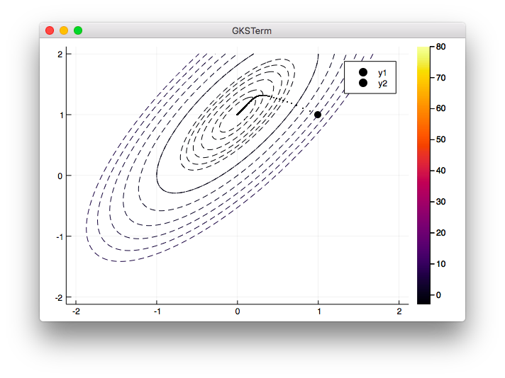
グラフを追加

Plotsパッケージを呼び出し、描画のロジックを追加します。

gd_test1.jl

using Plots
using .gd #自作Moduleは.付きで呼び出す

function f(xx::Array)
  x = xx[1]
  y = xx[2]
  5 * x^2 - 6 * x*y + 3 * y^2 + 6*x - 6*y
end

function df(xx::Array)
  x = xx[1]
  y = xx[2]
  [10 * x - 6 * y + 6, -6 * x + 6 * y - 6]
end

algo = gd.GradientDescent()
initial = [1, 1]
gd.solveGradientDescent(algo, f, df, initial)

println(algo.x_)
println(algo.opt_)

plt0 = scatter([initial[1]], [initial[2]], color="black", markersize=5)
plt1 = scatter!(plt0, algo.path_x_, algo.path_y_, color="black", markersize=1)

xs = LinRange(-2, 2, 300)
ys = LinRange(-2, 2, 300)

h(x,y) = f([x, y]) # 配列の形に直す
zs = h.(xs', ys)
levels = [-3, -2.9, -2.8, -2.6, -2.4, -2.2, -2, -1, -1, 0, 1, 2, 3, 4]

plot(plt1)
contour!(xs, ys, zs, levels=levels, color="black", linestyle=:dash)

実行結果

julia> include("gd.jl")
Main.gd

julia> include("gd_test1.jl")
[3.45723e-7, 1.0]
-2.9999999999997073

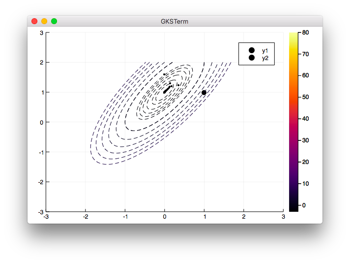
αの値を変える

ここは本ではαの値を[0.1, 0.2]と配列にしてfor文でグラフ表示しているのですが、どうしても同時に表示できませんでした。仕方がないので0.1と0.2用でコメントを入れ替えて表示しています。（グラフ表示はまだ自由に表現できず難航しています。）

0.1の時

gd_test2.jl

using Plots
using .gd

function f(xx::Array)
  x = xx[1]
  y = xx[2]
  5 * x^2 - 6 * x*y + 3 * y^2 + 6*x - 6*y
end

function df(xx::Array)
  x = xx[1]
  y = xx[2]
  [10 * x - 6 * y + 6, -6 * x + 6 * y - 6]
end

xmin = -3
xmax = 3
ymin = -3
ymax = 3

algos = []
initial = [1, 1]
alphas = [0.1, 0.2]

for α in alphas
  algo = gd.GradientDescent()
  gd.solveGradientDescent(algo, f, df, initial, α)
  push!(algos , algo)
end

xs = LinRange(-2, 2, 300)
ys = LinRange(-2, 2, 300)

h(x,y) = f([x, y]) # 配列の形に直す
zs = h.(xs', ys)
levels = [-3, -2.9, -2.8, -2.6, -2.4, -2.2, -2, -1, -1, 0, 1, 2, 3, 4]

plt0 = scatter([initial[1]], [initial[2]], color="black", markersize=5)

# 0.1の時用
plt1 = scatter!(plt0, algos[1].path_x_, algos[1].path_y_, color="black", markersize=1.5,xlim=(xmin, xmax), ylim=(ymin, ymax))

# 0.2の時用
# plt1 = scatter!(plt0, algos[2].path_x_, algos[2].path_y_, color="black", markersize=1.5,xlim=(xmin, xmax), ylim=(ymin, ymax))

plot(plt1)
contour!(xs, ys, zs, levels=levels, color="black", linestyle=:dash)

実行結果

julia> include("gd.jl")
Main.gd

julia> include("gd_test2.jl")

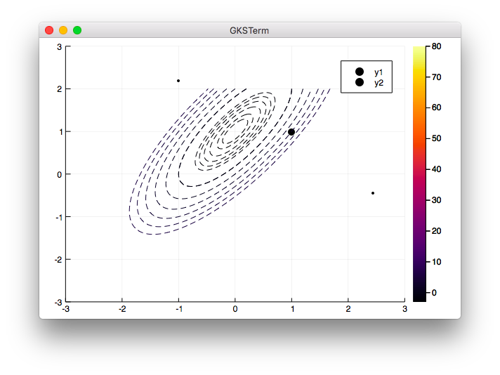
0.2の時

コメントを入れ替えます。

gd_test2.jl

（略）
# 0.1の時用
#plt1 = scatter!(plt0, algos[1].path_x_, algos[1].path_y_, color="black", markersize=1.5,xlim=(xmin, xmax), ylim=(ymin, ymax))

# 0.2の時用
plt1 = scatter!(plt0, algos[2].path_x_, algos[2].path_y_, color="black", markersize=1.5,xlim=(xmin, xmax), ylim=(ymin, ymax))
（略）

実行結果

julia> include("gd_test2.jl")

ニュートン法

1次元の場合

x^3 -5x + 1 = 0

newton1dim.jl

f(x) = x^3 - 5*x + 1

df(x) = 3*x^2 - 5

function newton1dim(f, df, x0, ϵ=1e-10, max_iter=1000)
  x = x0
  x_new = 0
  iter = 0
  while true
    x_new = x - f(x)/df(x)
    if abs(x - x_new ) < ϵ
      break
    end
    x = x_new
    iter += 1
    if iter == max_iter
      break
    end
  end
  return x_new
end

println(newton1dim(f, df, 2))
println(newton1dim(f, df, 0))
println(newton1dim(f, df, -3))

実行結果

julia> include("newton1dim.jl")
2.1284190638445772
0.20163967572340463
-2.330058739567982

• ϵ=eps()にした場合

勾配降下法のところではϵ=eps()にしたところ計算に時間がかかりすぎて結果が返ってこなかったのですが、ニュートン法ではすぐに結果が返ってきました。

julia> include("newton1dim.jl")
2.1284190638445772
0.20163967572340466
-2.330058739567982

0の時だけ少し数値が変わりました。

多次元の場合

\begin{eqnarray}
\left\{
\begin{array}{l}
f_1(x, y) &= x^3 -2y = 0 \\
f_2(x, y) &= x^2 + y^2 -1 = 0
\end{array}
\right.
\end{eqnarray}

まず計算のみ実装

• pathの保存は後で実装

newton.jl

module newton

struct Newton
  ϵ::Float64
  max_iter::Int

  function Newton(ϵ=1e-10, max_iter=1000)
    new(ϵ, max_iter)
  end
end

function solveNewton(newton::Newton, f, df, x0)
  x = x0
  x_new = 0
  iter = 0
  while true
    x_new = x - inv(df(x)) * f(x)
    if sum((x - x_new).^2) < (newton.ϵ)^2
      break
    end
    x = x_new
    iter += 1
    if iter == newton.max_iter
      break
    end
  end
  return x_new
end

end

• グラフの表示は後で実装

newton_test1.jl

using .newton

f1(x, y) = x^3 - 2*y
f2(x, y) = x^2 + y^2 -1

function f(xx)
  x = xx[1]
  y = xx[2]
  return [f1(x, y), f2(x, y)]
end

function df(xx)
  x = xx[1]
  y = xx[2]
  return [3*x^2 -2; 2*x 2*y]
end

solver = newton.Newton()
initials = [[1,1],[-1,-1],[1,-1]]
for x0 in initials
  sol = newton.solveNewton(solver, f, df, x0)
  println(sol)
end

実行結果

julia> include("newton.jl")
Main.newton

julia> include("newton_test1.jl")
[0.92071, 0.390247]
[-0.92071, -0.390247]
[-0.92071, -0.390247]

本と少し誤差はありますが、ほぼ同じ結果が得られました。

グラフを追加

pathを保存するように修正

newton.jl

module newton

mutable struct Newton
  ϵ::Float64
  max_iter::Int
  path_x_::Array
  path_y_::Array

  function Newton(ϵ=1e-10, max_iter=1000)
    new(ϵ, max_iter, [], [])
  end
end

function solveNewton(newton::Newton, f, df, x0)
  x = x0
  x_new = 0
  iter = 0
  push!(newton.path_x_, x0[1])
  push!(newton.path_y_, x0[2])
  while true
    x_new = x - inv(df(x)) * f(x)
    push!(newton.path_x_, x_new[1])
    push!(newton.path_y_, x_new[2])
    if sum((x - x_new).^2) < (newton.ϵ)^2
      break
    end
    x = x_new
    iter += 1
    if iter == newton.max_iter
      break
    end
  end
  return x_new
end

end

描画のロジックを追加。

• グラフの処理をfor文に入れると表示がどうしてもできなかったので、描画は最後にまとめて行うことにしました。

newton_test1.jl

using .newton
using Plots

f1(x, y) = x^3 - 2*y
f2(x, y) = x^2 + y^2 -1

function f(xx)
  x = xx[1]
  y = xx[2]
  return [f1(x, y), f2(x, y)]
end

function df(xx)
  x = xx[1]
  y = xx[2]
  return [3*x^2 -2; 2*x 2*y]
end

xmin = -3
xmax = 3
ymin = -3
ymax = 3

x = LinRange(xmin, xmax, 200)
y = LinRange(ymin, ymax, 200)

z1 = f1.(x',y)
z2 = f2.(x',y)

solver = newton.Newton()
initials = [[1,1],[-1,-1],[1,-1]]
solvers = []
for x0 in initials
  sol = newton.solveNewton(solver, f, df, x0)
  push!(solvers, solver)
  println(sol)
end

contour(x, y, z1, color="red", levels=[0], xlim=(xmin, xmax), ylim=(ymin, ymax))
contour!(x, y, z2, color="black", levels=[0])

scatter!(solvers[1].path_x_, solvers[1].path_y_, color="black", markershape=:+)
scatter!(solvers[2].path_x_, solvers[2].path_y_, color="black", markershape=:star8)
scatter!(solvers[3].path_x_, solvers[3].path_y_, color="black", markershape=:x)

実行結果

julia> include("newton.jl")
Main.newton

julia> include("newton_test1.jl")
[0.92071, 0.390247]
[-0.92071, -0.390247]
[-0.92071, -0.390247]

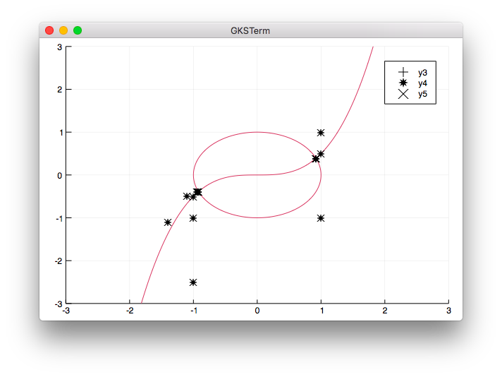
• 2番目のマーカー*がなかったので、star8で代替しています。星印です。
• z2のグラフ（楕円）の色はblackに指定したのですが、赤い色になってしまいました。

ラグランジュ未定乗数法

ここはサンプルがないので省略します。

Juliaの数理最適化ライブラリについて参考にしたサイト

JuMPライブラリについて・線形計画問題

• 最適化におけるJulia - JuMP事始め
• https://myenigma.hatenablog.com/entry/2017/07/31/025341
• http://www.juliaopt.org/JuMP.jl/0.17/quickstart.html

2次計画法

• http://ki-chi.jp/?p=895