【ラビットチャレンジ（E資格）】機械学習

はじめに

2021/2/19・20に実施される日本ディープラーニング協会(JDLA)Ｅ資格合格を目指して、ラビットチャレンジを受講した際の学習記録です。

科目一覧

応用数学
機械学習
深層学習（day1）
深層学習（day2）
深層学習（day3）
深層学習（day4）

第1章：線形回帰モデル

線形回帰（simple linear regression）

ひとつの予測変数によって、量的応答変数を予測する。
$$ \hat y = \hat{a}x+\hat{b} \quad　(\hat{a}：傾き, \hat{b}:切片) $$

• 学習データ $$ {(x_1,y_1),(x_2,y_2),…,(x_n,y_n)} $$
• （回帰）残差（residual） $$ e_i = y_i-\hat y_i $$
• 残差平方和（residual sum of squares, RSS） $$ \begin{align} RSS &= e_1^2 + e_2^2 + …e_n^2 \\ &= (y_1-\hat{b}-\hat{a}x_1)^2 + (y_2-\hat{b}-\hat{a}x_2)^2 + … + (y_n-\hat{b}-\hat{a}x_n)^2 \end{align}$$

最小二乗法により、平均二乗誤差（残差平方和）が最小になるようにパラメータを決める。
$$ \frac{\partial RSS}{\partial \hat{b}}=0, \quad \frac{\partial RSS}{\partial \hat{a}}=0 $$
$$ \hat{b} = \bar y-\hat{a}\bar x, \quad \hat{a}=\frac{\sum_{i=1}^n(x_i-\bar x)(y_i-\bar y)}{\sum_{i=1}^n(x_i-\bar x)^2}=\frac{Cov[x,y]}{Var[x]} $$

simple_linear_regression

import numpy as np
import matplotlib.pyplot as plt
%matplotlib inline

#データの作成
def linear_func(x):
    return 2 * x + 5

def add_noise(y_true, var):
    return y_true + np.random.normal(scale=var, size=y_true.shape)

n_sample = 100
var = .2

xs = np.linspace(0, 1, n_sample)
ys_true = linear_func(xs)
ys = add_noise(ys_true, var)

#学習
def train(xs, ys):
    cov = np.cov(xs, ys, ddof=0)
    a = cov[0, 1] / cov[0, 0]
    b = np.mean(ys) - a * np.mean(xs)
    return cov, a, b

cov, a, b = train(xs, ys)

#予測
xs_new = np.linspace(0, 1, n_sample)
ys_pred = a * xs_new + b

#結果の描画
plt.scatter(xs, ys, facecolor="none", edgecolor="b", s=50, label="training data")
plt.plot(xs_new, ys_true, label="$2 x + 5$")
plt.plot(xs_new, ys_pred, label="prediction (a={:.2}, b={:.2})".format(a, b))
plt.legend()
plt.show()

多重線形回帰（multiple linear regression）

複数の予測変数によって、量的応答変数を予測する。
$$ \begin{align}
\hat y &= \hat{w_0}+\hat{w_1}x_1+\hat{w_2}x_2+…+\hat{w_p}x_p \\
&= \sum_{j=1}^mw_jx_j + w_0 \\
&= w^\top x + w_0
\end{align} $$

• 残差平方和（residual sum of squares, RSS） $$ \begin{align} RSS &= \sum_{i=1}^n(y_i-\hat y_i)^2 \\ &= \sum_{i=1}^n(y_i-\hat{w_0}-\hat{w_1}x_{i1}+\hat{w_2}x_{i2}-…-\hat{w_p}x_{ip})^2 \end{align} $$

最小二乗法により、平均二乗誤差（残差平方和）が最小になるようにパラメータを決める。
$$ \frac{\partial RSS}{\partial \hat{w}} = -2x^\top(y-wx)=0 $$
$$ \hat{w} = (x^\top x)^{-1}x^\top y $$

multiple_linear_regression

import numpy as np
import matplotlib.pyplot as plt
%matplotlib inline

#データの作成
def mul_linear_func(x):
    global ww
    ww = [1., 0.5, 2., 1.]
    return ww[0] + ww[1] * x[:, 0] + ww[2] * x[:, 1] + ww[3] * x[:, 2]
def add_noise(y_true, var):
    return y_true + np.random.normal(scale=var, size=y_true.shape)

n_sample = 100
x_dim = 3
var = .2

X = np.random.random((n_sample, x_dim))
ys_true = mul_linear_func(X)
ys = add_noise(ys_true, var)

#学習
def add_one(x):
    return np.concatenate([np.ones(len(x))[:, None], x], axis=1)
X_train = add_one(X)
pinv = np.dot(np.linalg.inv(np.dot(X_train.T, X_train)), X_train.T)
w = np.dot(pinv, ys)

# 予測
def predict(w, x):
    return np.dot(w.T, x)
y_pred = predict(X_train.T, w)

第2章：非線形回帰モデル

基底展開法
- 回帰関数として、基底関数と呼ばれる既知の非線形関数とパラメータベクトルの線形結合を使用
- 未知パラメータは線形回帰モデルと同様に最小二乗法や最尤法により推定
$$ y_i = w_0 + \sum_{j=1}^mw_j\Phi_j(x_i) + \epsilon_i $$
$$ \hat{y} = \Phi (\Phi^{(train)\top} \Phi^{(train)})^{-1}\Phi^{(train)\top}y^{(train)} $$

よく使われる基底関数

• 多項式関数
  $$ \Phi_j = x^j $$

• ガウス型基底関数
  $$ \Phi_j(x) = \exp\Bigl\{\frac{(x-\mu_j)^2}{2h_j}\Bigl\} $$

• スプライン関数/Bスプライン関数

未学習（underfitting）

学習データに対して、十分小さな誤差が得られないモデル
対策:モデルの表現力が低いため、表現力の高いモデルを利用する

過学習（overfitting）

学習データに対して小さな誤差は得られたが、テストデータに対して誤差が大きいモデル
対策1:学習データの数を増やす
対策2:不要な基底関数を削除して表現力を抑止する

• 基底関数の数、位置やバンド幅によりモデルの複雑さが変化
• 解きたい問題に対して多くの基底関数を用意してしまうと過学習が起こるため、適切な基底関数を用意（CVなどで選択）

対策3:正則化法を利用して表現力を抑止する

• 「モデルの複雑さに伴って、その値が大きくなる正則化項（罰則化項）を課した関数」を最小化

• L2ノルムを利用:Ridge推定量（縮小推定…パラメータを0に近づけるよう推定）
  $$ \sum_{i=1}^n(y_i-\beta_0-\sum_{j=1}^p\beta_jx_{ij})^2 + \lambda\sum_{j=1}^p\beta_j^2 $$
  $\lambda$：ハイパーパラメータ

  • $\lambda$がゼロであれば最小二乗法と同じ
  • $\lambda$を大きくすると$\beta_1,…,\beta_p$は0に近づく（$\beta_0$にはペナルティがつかないことに注意）
  • 交差検証などによって適切な値に決める

• L1ノルムを利用:Lasso（the Least absolute shrinkage and selection operator）推定量（スパース推定…いくつかのパラメータを正確に0に推定）
  $$ \sum_{i=1}^n(y_i-\beta_0-\sum_{j=1}^p\beta_jx_{ij})^2 + \lambda\sum_{j=1}^p|\beta_j| $$

  • パラメータのL1ノルムに比例するペナルティ
  • $\lambda$ を大きくすると多くのパラメータが0になる 　$\rightarrow$変数選択によるスパースなモデルを生成

nonlinear_regression

import numpy as np
import matplotlib.pyplot as plt
%matplotlib inline

#データの作成
def true_func(x):
    z = 1-48*x+218*x**2-315*x**3+145*x**4
    return z 

def linear_func(x):
    z = x
    return z 

n = 100

# 真の関数からノイズを伴うデータを生成
# 真の関数からデータ生成
data = np.random.rand(n).astype(np.float32)
data = np.sort(data)
target = true_func(data)

# 　ノイズを加える
noise = 0.5 * np.random.randn(n) 
target = target  + noise

#線形回帰
from sklearn.linear_model import LinearRegression

clf = LinearRegression()
data = data.reshape(-1,1)
target = target.reshape(-1,1)
clf.fit(data, target)

p_lin = clf.predict(data)

#Ridge回帰
from sklearn.metrics.pairwise import rbf_kernel
from sklearn.linear_model import Ridge

kx = rbf_kernel(X=data, Y=data, gamma=50)

clf = Ridge(alpha=30)
clf.fit(kx, target)

p_ridge = clf.predict(kx)

#Lasso回帰
from sklearn.metrics.pairwise import rbf_kernel
from sklearn.linear_model import Lasso

kx = rbf_kernel(X=data, Y=data, gamma=5)

lasso_clf = Lasso(alpha=0.01, max_iter=1000)
lasso_clf.fit(kx, target)

p_lasso = lasso_clf.predict(kx)

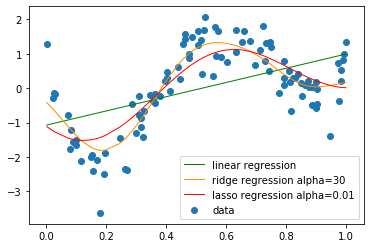
#結果の描画
plt.scatter(data, target, label='data')
plt.plot(data, p_lin, color='green', marker='', linestyle='-', linewidth=1, markersize=6, label='linear regression')
plt.plot(data, p_ridge, color='darkorange', linestyle='-', linewidth=1, markersize=6, label='ridge regression alpha=30')
plt.plot(data, p_lasso, color='red', linestyle='-', linewidth=1, markersize=6, label='lasso regression alpha=0.01')
plt.legend()

第3章：ロジスティック回帰（Logistic Regression）

線形回帰を分類問題に応用したアルゴリズム。
1. 対数オッズを重回帰分析により予測する
2. 対数オッズにロジット変換を施す（出力値が0から1の間の値に正規化される）ことで、クラス $i$ に属する確率 $pi$ の予測値を求める
3. 各クラスに属する確率を計算し、最大確率を実現するクラスが、データが属するクラスと予測する

$$ u = w^\top x + b $$

• ロジスティック関数を用いて確率値を計算 $$ p(X) = \frac{e^{\beta_0+\beta_1X}}{1+e^{\beta_0+\beta_1X}} = \frac{1}{1+e^{-(\beta_0+\beta_1X)}} $$
• オッズ（odds） $$ \frac{p(X)}{1-p(X)} = e^{\beta_0+\beta_1X} $$

• ロジット（logit, log-odds）
  $$ \log\Bigl(\frac{p(X)}{1-p(X)}\Bigl) = \beta_0+\beta_1X $$
  ロジットがXの線形関数になっている。

• 最尤推定（maximum likelihood estimation）
  尤度関数
  $$ L(w) = \prod_{n=1}^N\bigl({P(C_1|x_n)}\bigl)^{y_n} \bigl({1-P(C_1|x_n)}\bigl)^{1-y_n} $$
  が最大になるようにパラメータの値を決定する。

• 交差エントロピー（cross entropy）
  $$ E(w) = -\sum_{n=1}^N\Bigl(y_n\log{P(C_1|x_n)}+(1-y_n)\log\bigl({1-P(C_1|x_n)}\bigl)\Bigl) $$
  $L(w)$ の負の対数尤度で誤差関数を定義する。

logistic_regression

import numpy as np
import matplotlib.pyplot as plt
%matplotlib inline

#訓練データ生成
def gen_data(n_sample, harf_n_sample):
    x0 = np.random.normal(size=n_sample).reshape(-1, 2) - 1.
    x1 = np.random.normal(size=n_sample).reshape(-1, 2) + 1.
    x_train = np.concatenate([x0, x1])
    y_train = np.concatenate([np.zeros(harf_n_sample), np.ones(harf_n_sample)]).astype(np.int)
    return x_train, y_train

#データ作成
x_train, y_train = gen_data(n_sample, harf_n_sample)

n_sample = 100
harf_n_sample = 50
var = .2

#学習
def add_one(x):
    return np.concatenate([np.ones(len(x))[:, None], x], axis=1)

def sigmoid(x):
    return 1 / (1 + np.exp(-x))

def sgd(X_train, max_iter, eta):
    w = np.zeros(X_train.shape[1])
    for _ in range(max_iter):
        w_prev = np.copy(w)
        sigma = sigmoid(np.dot(X_train, w))
        grad = np.dot(X_train.T, (sigma - y_train))
        w -= eta * grad
        if np.allclose(w, w_prev):
            return w
    return w

X_train = add_one(x_train)
max_iter=100
eta = 0.01
w = sgd(X_train, max_iter, eta)

#予測
xx0, xx1 = np.meshgrid(np.linspace(-5, 5, 100), np.linspace(-5, 5, 100))
xx = np.array([xx0, xx1]).reshape(2, -1).T

X_test = add_one(xx)
proba = sigmoid(np.dot(X_test, w))
y_pred = (proba > 0.5).astype(np.int)

#結果の描画
plt.scatter(x_train[:, 0], x_train[:, 1], c=y_train)
plt.contourf(xx0, xx1, proba.reshape(100, 100), alpha=0.2, levels=np.linspace(0, 1, 3))

分類の評価方法

混同行列（confusion matrix）

• 再現率（Recall）、感度：Yesであるものを正しく検出できた割合 $$ \frac{TP}{TP+FN} $$
• 適合率（Precision）、精度：Yesと判定した中での正解率 $$ \frac{TP}{TP+FP} $$
• F値：再現率Rと適合率Pの調和平均 $$ \frac{2}{1/R+1/P} = \frac{2RP}{P+R} $$

第4章：主成分分析（Principle Component Analysis）

線形変換後の変数の分散が最大となる射影軸を探索することにより、多変量データの持つ構造をより少数個の指標に圧縮する。
$$ s_j = (s_{1j},…,s_{nj})^\top = \bar{X}a_j $$
$$ Var(s_j) = \frac{1}{n}s_j^Ts_j = \frac{1}{n}(\bar{X}a_j)^T(\bar{X}a_j) = \frac{1}{n}a_j^T\bar{X}^T\bar{X}a_j = a_j^TVar(\bar{X})a_j $$

• 以下の制約付き最適化問題を解く（ノルムが1という制約がないと、解が無限に存在してしまう）

$$ \text{目的関数} \qquad \arg \underset{a \in \mathbb{R}^m}{\textrm{max}} \; a_j^T Var(\bar{X})a_j $$
$$ \text{制約条件} \qquad a_j^Ta_j = 1 $$

• 制約付き最適化問題の解き方

ラグランジュ関数　$ E(a_j) = a_j^TVar(\bar{X})a_j - \lambda(a_j^Ta_j -1) $　を微分して最適解を求める。
$$ \frac{∂E(a_j)}{∂a_j} = 2Var(\bar{X})a_j - 2\lambda a_j = 0 $$
$$ Var(\bar{X})a_j = \lambda a_j $$
元のデータの分散共分散行列の固有値と固有ベクトルが、上記の制限付き最適化問題の解となる。
→　分散共分散行列の固有値と固有ベクトルを求めれば、分散を最大にする軸

• 寄与率（Proportion of variance explained, PVE）

元のデータの情報をどれだけ説明できているか。
$$ c_k \text{（第k主成分が持つ情報量）} = \frac{\lambda_k \text{（第k主成分の分散）}}{\sum_{i=1}^m \lambda_i \text{（主成分の総分散）}} $$

累積寄与率：第1~ $k$ 主成分まで圧縮した際の情報損失量の割合
$$ r_k \text{（第1} \sim \text{k主成分が持つ情報量）} = \frac{\sum_{j=1}^k \lambda_j \text{（第1} \sim \text{k主成分の分散）}}{\sum_{i=1}^m \lambda_i \text{（主成分の総分散）}} $$

principle_component_analysis

import numpy as np
import matplotlib.pyplot as plt
%matplotlib inline

#訓練データ生成
n_sample = 100

def gen_data(n_sample):
    mean = [0, 0]
    cov = [[2, 0.7], [0.7, 1]]
    return np.random.multivariate_normal(mean, cov, n_sample)

X = gen_data(n_sample)

#学習    
n_components=2

def get_moments(X):
    mean = X.mean(axis=0)
    stan_cov = np.dot((X - mean).T, X - mean) / (len(X) - 1)
    return mean, stan_cov

def get_components(eigenvectors, n_components):
#     W = eigenvectors[:, -n_components:]
#     return W.T[::-1]
    W = eigenvectors[:, ::-1][:, :n_components]
    return W.T

def plt_result(X, first, second):
    plt.scatter(X[:, 0], X[:, 1])
    plt.xlim(-5, 5)
    plt.ylim(-5, 5)
    # 第１主成分
    plt.quiver(0, 0, first[0], first[1], width=0.01, scale=6, color='red')
    # 第２主成分
    plt.quiver(0, 0, second[0], second[1], width=0.01, scale=6, color='green')

#分散共分散行列を標準化
meean, stan_cov = get_moments(X)
#固有値と固有ベクトルを計算
eigenvalues, eigenvectors = np.linalg.eigh(stan_cov)
components = get_components(eigenvectors, n_components)

#結果の描画
plt_result(X, eigenvectors[0, :], eigenvectors[1, :])

第5章：k近傍法（k-Nearest Neighbors）

最近傍のデータを$k$個取ってきて、それらが最も多く所属するクラスに識別する。
クラスの条件付き確率を推定
$$　Pr(Y=j|X=x_0) = \frac{1}{K}\sum_{i \in N_0}I(y_i = j) \qquad (N_0 \text{:学習データ中で} x_0 \text{に最も近い} K \text{個の観測データ}) $$

各クラスのデータ数の偏りがない、または各クラスがよく分かれているときしか精度が上がらないという弱点がある。

k-nearest_neighbors

import numpy as np
import matplotlib.pyplot as plt
from scipy import stats
%matplotlib inline

#訓練データ生成
def gen_data():
    x0 = np.random.normal(size=50).reshape(-1, 2) - 1
    x1 = np.random.normal(size=50).reshape(-1, 2) + 1.
    x_train = np.concatenate([x0, x1])
    y_train = np.concatenate([np.zeros(25), np.ones(25)]).astype(np.int)
    return x_train, y_train

X_train, ys_train = gen_data()

#予測
def distance(x1, x2):
    return np.sum((x1 - x2)**2, axis=1)

def knc_predict(n_neighbors, x_train, y_train, X_test):
    y_pred = np.empty(len(X_test), dtype=y_train.dtype)
    for i, x in enumerate(X_test):
        distances = distance(x, X_train)
        nearest_index = distances.argsort()[:n_neighbors]
        mode, _ = stats.mode(y_train[nearest_index])
        y_pred[i] = mode
    return y_pred

def plt_resut(x_train, y_train, y_pred):
    xx0, xx1 = np.meshgrid(np.linspace(-5, 5, 100), np.linspace(-5, 5, 100))
    xx = np.array([xx0, xx1]).reshape(2, -1).T
    plt.scatter(x_train[:, 0], x_train[:, 1], c=y_train)
    plt.contourf(xx0, xx1, y_pred.reshape(100, 100).astype(dtype=np.float), alpha=0.2, levels=np.linspace(0, 1, 3))

n_neighbors = 3

xx0, xx1 = np.meshgrid(np.linspace(-5, 5, 100), np.linspace(-5, 5, 100))
X_test = np.array([xx0, xx1]).reshape(2, -1).T

#結果の描画
y_pred = knc_predict(n_neighbors, X_train, ys_train, X_test)
plt_resut(X_train, ys_train, y_pred)

第6章：k-means（k平均法）

データを異なる $k$ 個のクラスタに分ける。
1. 各クラスタ中心の初期値を設定する。
2. 各データ点に対して、各クラスタ中心との距離を計算し、最も距離が近いクラスタを割り当てる。
3. 各クラスタの平均ベクトル（中心）を計算する。
4. 収束するまで2,3の処理を繰り返す。

k-means

import numpy as np
import matplotlib.pyplot as plt
%matplotlib inline

#データ生成
def gen_data():
    x1 = np.random.normal(size=(100, 2)) + np.array([-5, -5])
    x2 = np.random.normal(size=(100, 2)) + np.array([5, -5])
    x3 = np.random.normal(size=(100, 2)) + np.array([0, 5])
    return np.vstack((x1, x2, x3))

X_train = gen_data()

#学習
def distance(x1, x2):
    return np.sum((x1 - x2)**2, axis=1)

n_clusters = 3
iter_max = 100

# 各クラスタ中心をランダムに初期化
centers = X_train[np.random.choice(len(X_train), n_clusters, replace=False)]

for _ in range(iter_max):
    prev_centers = np.copy(centers)
    D = np.zeros((len(X_train), n_clusters))
    # 各データ点に対して、各クラスタ中心との距離を計算
    for i, x in enumerate(X_train):
        D[i] = distance(x, centers)
    # 各データ点に、最も距離が近いクラスタを割り当
    cluster_index = np.argmin(D, axis=1)
    # 各クラスタの中心を計算
    for k in range(n_clusters):
        index_k = cluster_index == k
        centers[k] = np.mean(X_train[index_k], axis=0)
    # 収束判定
    if np.allclose(prev_centers, centers):
        break

#クラスタリング結果
def plt_result(X_train, centers, xx):
    #　データを可視化
    plt.scatter(X_train[:, 0], X_train[:, 1], c=y_pred, cmap='spring')
    # 中心を可視化
    plt.scatter(centers[:, 0], centers[:, 1], s=200, marker='X', lw=2, c='black', edgecolor="white")
    # 領域の可視化
    pred = np.empty(len(xx), dtype=int)
    for i, x in enumerate(xx):
        d = distance(x, centers)
        pred[i] = np.argmin(d)
    plt.contourf(xx0, xx1, pred.reshape(100, 100), alpha=0.2, cmap='spring')

y_pred = np.empty(len(X_train), dtype=int)
for i, x in enumerate(X_train):
    d = distance(x, centers)
    y_pred[i] = np.argmin(d)

xx0, xx1 = np.meshgrid(np.linspace(-10, 10, 100), np.linspace(-10, 10, 100))
xx = np.array([xx0, xx1]).reshape(2, -1).T

#結果の描画
plt_result(X_train, centers, xx)

第7章：サポートベクターマシン（Support Vector Machine）

マージンが最大となる直線（パラメータ）を探す。

主問題の目的関数
$$ \text{min}_{w,b} \frac{1}{2}||w||^2 $$
制約条件
$$ t_i(w^\top x_i + b) \geq 1 \, (i=1,2,…,n) $$
上記の最適化問題をラグランジュ未定乗数法で解くことを考える。

• ラグランジュの未定乗数法
  制約付き最適化問題を解くための手法
  制約 $g_i(x) \geq 0 \, (i=1,2,…,n)$ のもとで、 $f(x)$ が最小となる $x$ は、変数 $\lambda_i \geq 0 \, (i=1,2,…,n)$ を用いて新たに定義したラグランジュ関数 $L(x,\lambda) = f(x)-\sum_{i=1}^n \lambda_i g(x)$において $\frac{\partial L}{\partial x_i} = 0 \, (j=1,2,…,m)$ を満たす。

• KNT条件
  制約付き最適化問題において最適解が満たす条件
  制約 $g_i(x) \geq 0 \, (i=1,2,…,n)$ のもとで、 $f(x)$ が最小となる $x^*$ は、以下の条件を満たす。

$$ \frac{\partial L}{\partial x_j}|x^* = 0 \, (j=1,2,…,m) $$
$$ g_i(x^*) \leq 0, \; \lambda_i \geq 0, \; \lambda_i g_i(x^*) = 0 \, (i=1,2,…,n) $$

線形分離可能

学習

特徴空間上で線形なモデル $y(x)= w \phi(x)+b$ を用い、その正負によって2値分類を行うことを考える。
サポートベクトターマシンではマージンの最大化を行うが、それは結局以下の最適化問題を解くことと同じである。
ただし、訓練データを $X=[x_1,x_2,…,x_n]^\top, t=[t_1,t_2,…,t_n]^\top \; (t_i=\{-1,+1\})$ とする。

$$ \text{min}_{w,b} \; \frac{1}{2}||w||^2 $$

$$ \text{subject to} \quad t_i(w\phi(x_i) + b) \ge 1 \; (i=1,2,…,n) $$

ラグランジュ乗数法を使うと、上の最適化問題はラグランジュ乗数$a \; (\ge 0)$を用いて、以下の目的関数を最小化する問題となる。

$$ L(w,b,a)=\frac{1}{2}||w||^2 - \sum_{i=1}^n a_i t_i(w \phi(x_i)+b-1) \qquad \cdots (1) $$

目的関数が最小となるのは、$w,b$ に関して偏微分した値が $0$ となるときなので、

$$ \frac{\partial L}{\partial w} = w-\sum_{i=1}^n a_i t_i \phi(x_i)=0 $$

$$ \frac{\partial L}{\partial b} = \sum_{i=1}^n a_i t_i = a^\top t = 0 $$

これを式(1)に代入することで、最適化問題は結局以下の目的関数の最大化となる。
$$ \begin{align}
\tilde{L}(a) &= \sum_{i=1}^{n} a_i - \frac{1}{2} \sum_{i=1}^n \sum_{j=1}^n a_i a_j t_i t_j \phi(x_i)^\top \phi(x_j) \\
&= a^\top - \frac{1}{2} a^\top H a
\end{align} $$

ただし、行列 $H$ の $i$ 行 $j$ 列成分は $H_{ij}=t_i t_j \phi(x_i)^\top \phi(x_j) = t_i t_j k(x_i,x_j)$である。
また制約条件は、$a^\top t = 0 \; (\frac{1}{2} || a^\top t ||^2 = 0)$ である。

この最適化問題を最急降下法で解く。目的関数と制約条件を $a$ で微分すると、
$$ \frac{\partial \tilde{L}}{\partial a} = 1 - Ha $$

$$ \frac{\partial}{\partial a} (\frac{1}{2} || a^\top t ||^2) = (a^\top t) t $$

なので、 $a$ を以下の二式で更新する。

$$ a \leftarrow a + \eta_1 (1 - Ha) $$

$$ a \leftarrow a - \eta_2 (a^\top t) t $$

予測

新しいデータ点 $x$ に対しては、$y(x)= w \phi(x)+b = \sum_{i=1}^n a_i t_i k(x, x_i)+b$ の正負によって分類する。

ここで、最適化の結果得られた $a_i (i=1,2,…,n)$ の中で $a_i=0$ に対応するデータ点は予測に影響を与えないので、 $a_i > 0$ に対応するデータ点（サポートベクトル）のみ保持しておく。
$b$ はサポートベクトルのインデックスの集合を $S$ とすると、 $b = \frac{1}{S} \sum_{s \in S} \bigl( t_s-\sum_{i=1}^n a_i t_i k(x_i,x_s) \bigl)$ によって求める。

support_vector_machine①

import numpy as np
import matplotlib.pyplot as plt
%matplotlib inline

#訓練データ生成（線形分離可能）
def gen_data():
    x0 = np.random.normal(size=50).reshape(-1, 2) - 2.
    x1 = np.random.normal(size=50).reshape(-1, 2) + 2.
    X_train = np.concatenate([x0, x1])
    ys_train = np.concatenate([np.zeros(25), np.ones(25)]).astype(np.int)
    return X_train, ys_train

X_train, ys_train = gen_data()

#学習
t = np.where(ys_train == 1.0, 1.0, -1.0)

n_samples = len(X_train)
# 線形カーネル
K = X_train.dot(X_train.T)

eta1 = 0.01
eta2 = 0.001
n_iter = 500

H = np.outer(t, t) * K

a = np.ones(n_samples)
for _ in range(n_iter):
    grad = 1 - H.dot(a)
    a += eta1 * grad
    a -= eta2 * a.dot(t) * t
    a = np.where(a > 0, a, 0)

#予測
index = a > 1e-6
support_vectors = X_train[index]
support_vector_t = t[index]
support_vector_a = a[index]

term2 = K[index][:, index].dot(support_vector_a * support_vector_t)
b = (support_vector_t - term2).mean()

xx0, xx1 = np.meshgrid(np.linspace(-5, 5, 100), np.linspace(-5, 5, 100))
xx = np.array([xx0, xx1]).reshape(2, -1).T

X_test = xx
y_project = np.ones(len(X_test)) * b
for i in range(len(X_test)):
    for a, sv_t, sv in zip(support_vector_a, support_vector_t, support_vectors):
        y_project[i] += a * sv_t * sv.dot(X_test[i])
y_pred = np.sign(y_project)

# 訓練データを可視化
plt.scatter(X_train[:, 0], X_train[:, 1], c=ys_train)
# サポートベクトルを可視化
plt.scatter(support_vectors[:, 0], support_vectors[:, 1],
                    s=100, facecolors='none', edgecolors='k')
# 領域を可視化
#plt.contourf(xx0, xx1, y_pred.reshape(100, 100), alpha=0.2, levels=np.linspace(0, 1, 3))
# マージンと決定境界を可視化
plt.contour(xx0, xx1, y_project.reshape(100, 100), colors='k',
                     levels=[-1, 0, 1], alpha=0.5, linestyles=['--', '-', '--'])

# マージンと決定境界を可視化
plt.quiver(0, 0, 0.1, 0.35, width=0.01, scale=1, color='pink')

線形分離不可能

学習

元のデータ空間では線形分離は出来ないが、特徴空間上で線形分離することを考える。
今回はカーネルとしてRBFカーネル（ガウシアンカーネル）を利用する。

support_vector_machine②

#訓練データ生成（線形分離不可能）
factor = .2
n_samples = 50
linspace = np.linspace(0, 2 * np.pi, n_samples // 2 + 1)[:-1]
outer_circ_x = np.cos(linspace)
outer_circ_y = np.sin(linspace)
inner_circ_x = outer_circ_x * factor
inner_circ_y = outer_circ_y * factor

X = np.vstack((np.append(outer_circ_x, inner_circ_x),
               np.append(outer_circ_y, inner_circ_y))).T
y = np.hstack([np.zeros(n_samples // 2, dtype=np.intp),
               np.ones(n_samples // 2, dtype=np.intp)])
X += np.random.normal(scale=0.15, size=X.shape)
x_train = X
y_train = y

#学習
def rbf(u, v):
        sigma = 0.8
        return np.exp(-0.5 * ((u - v)**2).sum() / sigma**2)

X_train = x_train
t = np.where(y_train == 1.0, 1.0, -1.0)

n_samples = len(X_train)
# RBFカーネル
K = np.zeros((n_samples, n_samples))
for i in range(n_samples):
    for j in range(n_samples):
        K[i, j] = rbf(X_train[i], X_train[j])

eta1 = 0.01
eta2 = 0.001
n_iter = 5000

H = np.outer(t, t) * K

a = np.ones(n_samples)
for _ in range(n_iter):
    grad = 1 - H.dot(a)
    a += eta1 * grad
    a -= eta2 * a.dot(t) * t
    a = np.where(a > 0, a, 0)

#予測
index = a > 1e-6
support_vectors = X_train[index]
support_vector_t = t[index]
support_vector_a = a[index]

term2 = K[index][:, index].dot(support_vector_a * support_vector_t)
b = (support_vector_t - term2).mean()

xx0, xx1 = np.meshgrid(np.linspace(-1.5, 1.5, 100), np.linspace(-1.5, 1.5, 100))
xx = np.array([xx0, xx1]).reshape(2, -1).T

X_test = xx
y_project = np.ones(len(X_test)) * b
for i in range(len(X_test)):
    for a, sv_t, sv in zip(support_vector_a, support_vector_t, support_vectors):
        y_project[i] += a * sv_t * rbf(X_test[i], sv)
y_pred = np.sign(y_project)

# 訓練データを可視化
plt.scatter(x_train[:, 0], x_train[:, 1], c=y_train)
# サポートベクトルを可視化
plt.scatter(support_vectors[:, 0], support_vectors[:, 1],
                    s=100, facecolors='none', edgecolors='k')
# 領域を可視化
plt.contourf(xx0, xx1, y_pred.reshape(100, 100), alpha=0.2, levels=np.linspace(0, 1, 3))
# マージンと決定境界を可視化
plt.contour(xx0, xx1, y_project.reshape(100, 100), colors='k',
                     levels=[-1, 0, 1], alpha=0.5, linestyles=['--', '-', '--'])

ソフトマージンSVM

• サンプルを線形分離できないとき、誤差を許容し、誤差に対してペナルティを与える
• パラメータ $C$ の大小で決定境界が変化
  • $C$ が小さいとき→誤差をより許容する
  • $C$ が大きいとき→誤差をあまり許容しない

目的関数
$$ \frac{1}{2}||w||^2 + C \sum_{i=1}^n \xi_i $$
制約条件
$$ t_i(w^\top x_i + b) \geq 1-\xi_i, \, \xi_i \geq 0 $$

学習

分離不可能な場合は学習できないが、データ点がマージン内部に入ることや誤分類を許容することでその問題を回避する。

スラック変数 $\xi_{i} \ge 0$ を導入し、マージン内部に入ったり誤分類された点に対しては、$\xi_{i} = |1 - t_{i} y(x_i)|$とし、これらを許容する代わりに対して、ペナルティを与えるように、最適化問題を以下のように修正する。

$$ min_{w,b} \qquad \frac{1}{2} ||w||^2 + \sum_{i=1}^n \xi_i $$

$$ \text{subject to} \qquad t_i(w \phi(x_i)+b) \ge 1 - \xi_{i} \; (i=1,2,…,n) $$

ただし、パラメータ$C$はマージンの大きさと誤差の許容度のトレードオフを決めるパラメータである。
この最適化問題をラグランジュ乗数法などを用いると、結局最大化する目的関数はハードマージンSVMと同じとなる。

$$ \tilde{L}(a) = \sum_{i=1}^n a_i - \frac{1}{2} \sum_{i=1}^n \sum_{j=1}^n a_i a_j t_i t_j \phi(x_i)^\top \phi(x_j) $$

ただし、制約条件が $a_{i} \ge 0$の代わりに$0 \le a_{i} \le C (i = 1, 2, ..., n)$ となる。（ハードマージンSVMと同じ $\sum_{i=1}^{n} a_{i} t_{i} = 0$ も制約条件）

support_vector_machine③

#訓練データ生成（重なりあり）
x0 = np.random.normal(size=50).reshape(-1, 2) - 1.
x1 = np.random.normal(size=50).reshape(-1, 2) + 1.
x_train = np.concatenate([x0, x1])
y_train = np.concatenate([np.zeros(25), np.ones(25)]).astype(np.int)

#学習
X_train = x_train
t = np.where(y_train == 1.0, 1.0, -1.0)

n_samples = len(X_train)
# 線形カーネル
K = X_train.dot(X_train.T)

C = 1
eta1 = 0.01
eta2 = 0.001
n_iter = 1000

H = np.outer(t, t) * K

a = np.ones(n_samples)
for _ in range(n_iter):
    grad = 1 - H.dot(a)
    a += eta1 * grad
    a -= eta2 * a.dot(t) * t
    a = np.clip(a, 0, C)

#予測
index = a > 1e-8
support_vectors = X_train[index]
support_vector_t = t[index]
support_vector_a = a[index]

term2 = K[index][:, index].dot(support_vector_a * support_vector_t)
b = (support_vector_t - term2).mean()

xx0, xx1 = np.meshgrid(np.linspace(-4, 4, 100), np.linspace(-4, 4, 100))
xx = np.array([xx0, xx1]).reshape(2, -1).T

X_test = xx
y_project = np.ones(len(X_test)) * b
for i in range(len(X_test)):
    for a, sv_t, sv in zip(support_vector_a, support_vector_t, support_vectors):
        y_project[i] += a * sv_t * sv.dot(X_test[i])
y_pred = np.sign(y_project)

# 訓練データを可視化
plt.scatter(x_train[:, 0], x_train[:, 1], c=y_train)
# サポートベクトルを可視化
plt.scatter(support_vectors[:, 0], support_vectors[:, 1],
                    s=100, facecolors='none', edgecolors='k')
# 領域を可視化
plt.contourf(xx0, xx1, y_pred.reshape(100, 100), alpha=0.2, levels=np.linspace(0, 1, 3))
# マージンと決定境界を可視化
plt.contour(xx0, xx1, y_project.reshape(100, 100), colors='k',
                     levels=[-1, 0, 1], alpha=0.5, linestyles=['--', '-', '--'])