概要
- DataExplorerは探索的データ解析を手助けするR言語のパッケージ
- ggplot2パッケージをラップしており、関数ひとつでデータセットを可視化できる
- 可視化結果をまとめたHTML形式の定型レポート生成も手軽
前書き
探索的データ解析(EDA: Exploratory Data Analysis)とは?
S-PLUS -トップ > 製品概要 > 探索的データ解析」より引用。
探索的データ解析は、1960年ごろより有名な統計学者J.W.Tukeyによって提唱されたもので、データの解釈にあたっては「まずモデルありき」ではなく、モデルを仮定する前に現実的な立場で、データの示唆する情報を多面的に捉えるという、解析初期のフェーズを重視したアプローチです。
それ以前は、あらかじめモデルを用意して、データをあてはめて確率計算を行っていました。しかし現実には、複雑な現実のデータ構造の中から、最適なモデルをあらかじめ用意することは簡単なことではありません。そのため、データを見てからモデルを修正したり、選択する必要が発生します。
また、数理統計学の理論的側面よりもむしろ、あくまでも応用面と結びついた、やさしく誰でも使えるような手法を重視しているために、ビジネスの現場での「データマイニング」などにも有効に活用できるアプローチといえるでしょう。
事前に読んでおくと良い記事。
背景
データセットの集計が間違っていたり、どういうデータでどういう意図で作ったかなどの説明もほとんどなくとりあえずデータを渡したりする分析依頼は数多くあります。このような案件はデータの検証や理解から進める必要があり、丁寧な統計モデリングや機械学習で効果を出すまでに時間がかかります。そういった分析に対する無理解は担当者の退職に繋がるかもしれません。
こういった状況を避けるためには、ドキュメント整備やデータセットの状態をモニタリング、探索的データ解析の結果をまとめて共有するなど、情報や知見をチームや組織に貯めていくのが肝要になります。
中でも探索的データ解析はデータを理解した仮説の立案と磨き上げができる重要なタスクです。基礎分析や可視化が多く誰にでもできる単純作業と見なされがちですが、データを正しく処理する知識とスキル、適した仮説を立てるセンスを要します(センスは対象となるデータとビジネスの理解によって、ある程度は補完できます)。
システムにあったバグやユーザーの不適切な行動をデータから発見するケースもあり、ビジネスの現場で気づいていなかった有用な仮説が生まれるときもあります。
とはいえ業務としては見つけるだけがゴールではなく、共通化・自動化できる部分はシステム化して負荷軽減を考える必要もあります。
DataExplorerパッケージは「探索的データ解析」「特徴量エンジニアリング」「レポーティング」の各タスクを手軽にするパッケージで、中でも探索的データ解析を補助する可視化関連の関数群が多く定義されています。これらを用いるとデータセットの傾向を手早く把握できます。
本記事ではDataExplorerパッケージの関数を実際に動かして挙動を確認しながら説明します。
- DataExplorer: Automate Data Exploration and Treatment (CRAN)
- Introduction to DataExplorer (CRAN - Vignettes)
- DataExplorer: Automate Data Exploration and Treatment (GitHub)
また、GitHubリポジトリにあるWikiにはDataExplorerパッケージを使用したブログや記事などがまとめられています。利用例が知りたい方はご参考ください。
共通
本記事ではDataExplorerパッケージの使い方を説明しますが、その際に必要となる定数や共通利用される関数定義をここでは行います。
また、本筋とそれますが「ソース内で参照するパッケージの一覧」を取得する方法に関しても記載しています。
options(repos = c(CRAN = "https://cran.ism.ac.jp/"))
options(tidyverse.quiet = TRUE)

# patchworkは可視化用
LOAD_PKGS <- c("tidyverse", "DataExplorer", "patchwork")

# patchworkパッケージはまでCRANに上がっていない
# remotes::install_github(repo = "thomasp85/patchwork")
# 「tidyr::pivot_*」を使う
# remotes::install_github(repo = "tidyverse/tidyr", upgrade = "always")
pacman::p_load(LOAD_PKGS, install = FALSE, character.only = TRUE)


# 指定パッケージの関数毎に名前空間を返す
# 演算子などはパターンを用いて除く
# pacman::p_funsは別パッケージからのロードされた関数かどうか区別がつかないので使わない
tidyPkgNamespace <- function(
  pkg_name, var_nm = "function_name", exclude_pattern = "(%)|(\\<-)|(\\=)|(\\!)"
) {
  lsf.str(
    pos = glue::glue("package:{pkg_name}", pkg_name = pkg_name), all = TRUE
  ) %>%
    unclass() %>%
    as.character() %>%
    tibble::enframe(name = NULL, value = var_nm) %>%
    dplyr::filter(
      stringr::str_detect(
        string = !!rlang::sym(x = var_nm),
        pattern = exclude_pattern, negate = TRUE
      )
    ) %>%
    dplyr::group_by(!!rlang::sym(x = var_nm)) %>%
    dplyr::summarize(
      ns = as.character(
        x = environmentName(
          env = rlang::fn_env(
            fn = rlang::as_closure(x = !!rlang::sym(x = var_nm))
          )
        )
      )
    ) %>%
    return()
}
ソース内で使用しているパッケージ一覧
Dockerfile作成やパッケージ開発はもちろん、ブログ記事でもRのソースコードファイル内で呼び出しているパッケージの一覧が欲しくなるときがあります。
ここでは「ソース内で参照するパッケージの一覧表示」をattachmentパッケージを利用して取得しており、これによって上記のような「まとめて読み込む部分以外でパッケージを呼び出し、忘れた頃に実行したら必要パッケージが洩れていた」という事態がなくなります。
# 基本パッケージやtidyverse依存パッケージなどは除く
dplyr::setdiff(
  # rstudioapiはRStudio上で実行する場合のみ
  # https://github.com/rstudio/rstudioapi/issues/7
  x = attachment::att_from_rmd(path = rstudioapi::getSourceEditorContext()$path),
  y = c(
    # 環境情報などに関するパッケージも除外
    c("attachment", "pacman", "sessioninfo"),
    # 基本パッケージ
    installed.packages() %>% tibble::as_tibble() %>%
      dplyr::filter(!is.na(x = Priority)) %>% dplyr::pull(var = "Package"),
    # tidyverse
    tidyverse::tidyverse_deps(recursive = TRUE) %>% dplyr::pull(var = "package")
    )
)
# > [1] "tidyverse"    "DataExplorer" "patchwork"
また、R言語の実行環境を再現する方法には以下のようなDockerイメージ作成・パッケージ管理などもありますが、ある程度の慣れや知見が必要となりますのでattachmentパッケージのattachment::att_from_rmds()やattachment::att_from_rscripts()で使用しているパッケージの一覧を得るから始めるのも良いでしょう。
個人的にはrenvパッケージの今後のご活躍を期待しております。
- packrat: A Dependency Management System for Projects and their R Package Dependencies (CRAN)
- miniCRAN: Create a Mini Version of CRAN Containing Only Selected Packages (CRAN)
- Package an R workspace and all dependencies as a Docker container (GitHub)
- renv: Project environments for R (GitHub)
関数一覧
DataExplorerパッケージが提供している関数(別パッケージからのロードは除く)は次の通りです。主に各種可視化を行う関数群が「plot_*」の名称によって定義されています。
data_explorer_functions <- tidyPkgNamespace(pkg_name = "DataExplorer") %>%
  print(n = Inf)
# > # A tibble: 22 x 2
# >    function_name    ns
# >    <chr>            <chr>
# >  1 configure_report DataExplorer
# >  2 create_report    DataExplorer
# >  3 drop_columns     DataExplorer
# >  4 dummify          DataExplorer
# >  5 group_category   DataExplorer
# >  6 introduce        DataExplorer
# >  7 plot_bar         DataExplorer
# >  8 plot_boxplot     DataExplorer
# >  9 plot_correlation DataExplorer
# > 10 plot_density     DataExplorer
# > 11 plot_histogram   DataExplorer
# > 12 plot_intro       DataExplorer
# > 13 plot_missing     DataExplorer
# > 14 plot_prcomp      DataExplorer
# > 15 plot_qq          DataExplorer
# > 16 plot_scatterplot DataExplorer
# > 17 plot_str         DataExplorer
# > 18 plotDataExplorer DataExplorer
# > 19 profile_missing  DataExplorer
# > 20 set_missing      DataExplorer
# > 21 split_columns    DataExplorer
# > 22 update_columns   DataExplorer
# 全関数がDataExplorerパッケージ由来
data_explorer_functions %>% dplyr::add_tally(name = "rows") %>%
  dplyr::group_by(ns, rows) %>% dplyr::tally(name = "func_count")
# > # A tibble: 1 x 3
# > # Groups:   ns [1]
# >   ns            rows func_count
# >   <chr>        <int>      <int>
# > 1 DataExplorer    22         22
# dplyrはrlang, tibble, tidyselectなどからインポートされた関数を含む
# tidyPkgNamespace(pkg_name = "dplyr") %>% dplyr::group_by(ns) %>% dplyr::tally()


# 解説関数確認用
data_explorer_funs_vari <- tibble::tibble(function_name = character())
一覧で確認したDataExplorerパッケージの関数群を以下のように分けて、本記事ではこの区分で説明します。
- データセットの構造を可視化
- plot_str
- データセットの情報を可視化
- introduce/plot_intro
- profile_missing/plot_missing
- データセット中にある変数の情報を可視化
- plot_bar
- plot_scatterplot/plot_boxplot/plot_density/plot_histogram
- plot_correlation/plot_prcomp/plot_qq
- 特徴量エンジニアリング
- dummify/group_category
- レポート生成
- configure_report/create_report
- ユーティリティ関数
- plotDataExplorer
- split_columns
- drop_columns/update_columns/set_missing
関数解説
DataExplorerパッケージが提供している関数について、実際に動かして挙動を確認しながら前節の区分毎に説明します。
解説対象とする区分は「データセットの構造を可視化」、「データセットの情報を可視化」、「データセット中にある変数の情報を可視化」、「特徴量エンジニアリング」、ならびに「ユーティリティ関数」の一部です。
本記事で触れていない関数は「飛ばした関数」の項目にまとめておりますので、興味がある方は随時ご確認ください。
データセットの構造を可視化
Rオブジェクトのデータ構造を把握するための関数にutils::str()やtibble::glimpse()があります。
これらは構造がわからない関数の戻り値やデータセットに適用して確認する際に用いますが、複雑さが増した結果には向きません。
# str()
str(object = datasets::iris)
# > 'data.frame':    150 obs. of  5 variables:
# >  $ Sepal.Length: num  5.1 4.9 4.7 4.6 5 5.4 4.6 5 4.4 4.9 ...
# >  $ Sepal.Width : num  3.5 3 3.2 3.1 3.6 3.9 3.4 3.4 2.9 3.1 ...
# >  $ Petal.Length: num  1.4 1.4 1.3 1.5 1.4 1.7 1.4 1.5 1.4 1.5 ...
# >  $ Petal.Width : num  0.2 0.2 0.2 0.2 0.2 0.4 0.3 0.2 0.2 0.1 ...
# >  $ Species     : Factor w/ 3 levels "setosa","versicolor",..: 1 1 1 1 1 1 1 1 1 1 ...

# glimpse()
datasets::iris %>% tibble::glimpse()
# > Observations: 150
# > Variables: 5
# > $ Sepal.Length <dbl> 5.1, 4.9, 4.7, 4.6, 5.0, 5.4, 4.6, 5.0, 4.4, 4.9, …
# > $ Sepal.Width  <dbl> 3.5, 3.0, 3.2, 3.1, 3.6, 3.9, 3.4, 3.4, 2.9, 3.1, …
# > $ Petal.Length <dbl> 1.4, 1.4, 1.3, 1.5, 1.4, 1.7, 1.4, 1.5, 1.4, 1.5, …
# > $ Petal.Width  <dbl> 0.2, 0.2, 0.2, 0.2, 0.2, 0.4, 0.3, 0.2, 0.2, 0.1, …
# > $ Species      <fct> setosa, setosa, setosa, setosa, setosa, setosa, se…

# glimpse()はパイプ演算子で処理が続けられる
ggplot2::diamonds %>% tibble::glimpse() %>% dplyr::filter(cut == "Premium")
# > Observations: 53,940
# > Variables: 10
# > $ carat   <dbl> 0.23, 0.21, 0.23, 0.29, 0.31, 0.24, 0.24, 0.26, 0.22, 0…
# > $ cut     <ord> Ideal, Premium, Good, Premium, Good, Very Good, Very Go…
# > $ color   <ord> E, E, E, I, J, J, I, H, E, H, J, J, F, J, E, E, I, J, J…
# > $ clarity <ord> SI2, SI1, VS1, VS2, SI2, VVS2, VVS1, SI1, VS2, VS1, SI1…
# > $ depth   <dbl> 61.5, 59.8, 56.9, 62.4, 63.3, 62.8, 62.3, 61.9, 65.1, 5…
# > $ table   <dbl> 55, 61, 65, 58, 58, 57, 57, 55, 61, 61, 55, 56, 61, 54,…
# > $ price   <int> 326, 326, 327, 334, 335, 336, 336, 337, 337, 338, 339, …
# > $ x       <dbl> 3.95, 3.89, 4.05, 4.20, 4.34, 3.94, 3.95, 4.07, 3.87, 4…
# > $ y       <dbl> 3.98, 3.84, 4.07, 4.23, 4.35, 3.96, 3.98, 4.11, 3.78, 4…
# > $ z       <dbl> 2.43, 2.31, 2.31, 2.63, 2.75, 2.48, 2.47, 2.53, 2.49, 2…
# > # A tibble: 13,791 x 10
# >    carat cut     color clarity depth table price     x     y     z
# >    <dbl> <ord>   <ord> <ord>   <dbl> <dbl> <int> <dbl> <dbl> <dbl>
# >  1 0.21  Premium E     SI1      59.8    61   326  3.89  3.84  2.31
# >  2 0.290 Premium I     VS2      62.4    58   334  4.2   4.23  2.63
# >  3 0.22  Premium F     SI1      60.4    61   342  3.88  3.84  2.33
# >  4 0.2   Premium E     SI2      60.2    62   345  3.79  3.75  2.27
# >  5 0.32  Premium E     I1       60.9    58   345  4.38  4.42  2.68
# >  6 0.24  Premium I     VS1      62.5    57   355  3.97  3.94  2.47
# >  7 0.290 Premium F     SI1      62.4    58   403  4.24  4.26  2.65
# >  8 0.22  Premium E     VS2      61.6    58   404  3.93  3.89  2.41
# >  9 0.22  Premium D     VS2      59.3    62   404  3.91  3.88  2.31
# > 10 0.3   Premium J     SI2      59.3    61   405  4.43  4.38  2.61
# > # … with 13,781 more rows


# 複雑な構造のリスト例
nested_list <- list(
  a = list(
    iris = datasets::iris, airquality = datasets::airquality,
    list(mtcars = datasets::mtcars, USArrests = datasets::USArrests)
  ),
  b = list(
    time_series = list(ts(data = seq_len(length.out = 10), frequency = 4))
  ),
  c = lm(formula = rnorm(n = 5) ~ seq_len(length.out = 5)),
  d = lapply(
    X = seq_len(length.out = 5),
    FUN = function(x) {
      return(as.function(x = function(y) {
        return(y + 1)
      }))
    }
  )
)

# よくわからなくなる
str(object = nested_list)
# > List of 4
# >  $ a:List of 3
# >   ..$ iris      :'data.frame':   150 obs. of  5 variables:
# >   .. ..$ Sepal.Length: num [1:150] 5.1 4.9 4.7 4.6 5 5.4 4.6 5 4.4 4.9 ...
# >   .. ..$ Sepal.Width : num [1:150] 3.5 3 3.2 3.1 3.6 3.9 3.4 3.4 2.9 3.1 ...
# >   .. ..$ Petal.Length: num [1:150] 1.4 1.4 1.3 1.5 1.4 1.7 1.4 1.5 1.4 1.5 ...
# >   .. ..$ Petal.Width : num [1:150] 0.2 0.2 0.2 0.2 0.2 0.4 0.3 0.2 0.2 0.1 ...
# >   .. ..$ Species     : Factor w/ 3 levels "setosa","versicolor",..: 1 1 1 1 1 1 1 1 1 1 ...
# >   ..$ airquality:'data.frame':   153 obs. of  6 variables:
# >   .. ..$ Ozone  : int [1:153] 41 36 12 18 NA 28 23 19 8 NA ...
# >   .. ..$ Solar.R: int [1:153] 190 118 149 313 NA NA 299 99 19 194 ...
# >   .. ..$ Wind   : num [1:153] 7.4 8 12.6 11.5 14.3 14.9 8.6 13.8 20.1 8.6 ...
# >   .. ..$ Temp   : int [1:153] 67 72 74 62 56 66 65 59 61 69 ...
# >   .. ..$ Month  : int [1:153] 5 5 5 5 5 5 5 5 5 5 ...
# >   .. ..$ Day    : int [1:153] 1 2 3 4 5 6 7 8 9 10 ...
# >   ..$           :List of 2
# >   .. ..$ mtcars   :'data.frame': 32 obs. of  11 variables:
# >   .. .. ..$ mpg : num [1:32] 21 21 22.8 21.4 18.7 18.1 14.3 24.4 22.8 19.2 ...
# >   .. .. ..$ cyl : num [1:32] 6 6 4 6 8 6 8 4 4 6 ...
# >   .. .. ..$ disp: num [1:32] 160 160 108 258 360 ...
# >   .. .. ..$ hp  : num [1:32] 110 110 93 110 175 105 245 62 95 123 ...
# >   .. .. ..$ drat: num [1:32] 3.9 3.9 3.85 3.08 3.15 2.76 3.21 3.69 3.92 3.92 ...
# >   .. .. ..$ wt  : num [1:32] 2.62 2.88 2.32 3.21 3.44 ...
# >   .. .. ..$ qsec: num [1:32] 16.5 17 18.6 19.4 17 ...
# >   .. .. ..$ vs  : num [1:32] 0 0 1 1 0 1 0 1 1 1 ...
# >   .. .. ..$ am  : num [1:32] 1 1 1 0 0 0 0 0 0 0 ...
# >   .. .. ..$ gear: num [1:32] 4 4 4 3 3 3 3 4 4 4 ...
# >   .. .. ..$ carb: num [1:32] 4 4 1 1 2 1 4 2 2 4 ...
# >   .. ..$ USArrests:'data.frame': 50 obs. of  4 variables:
# >   .. .. ..$ Murder  : num [1:50] 13.2 10 8.1 8.8 9 7.9 3.3 5.9 15.4 17.4 ...
# >   .. .. ..$ Assault : int [1:50] 236 263 294 190 276 204 110 238 335 211 ...
# >   .. .. ..$ UrbanPop: int [1:50] 58 48 80 50 91 78 77 72 80 60 ...
# >   .. .. ..$ Rape    : num [1:50] 21.2 44.5 31 19.5 40.6 38.7 11.1 15.8 31.9 25.8 ...
# >  $ b:List of 1
# >   ..$ time_series:List of 1
# >   .. ..$ : Time-Series [1:10] from 1 to 3.25: 1 2 3 4 5 6 7 8 9 10
# >  $ c:List of 12
# >   ..$ coefficients : Named num [1:2] -1.577 0.222
# >   .. ..- attr(*, "names")= chr [1:2] "(Intercept)" "seq_len(length.out = 5)"
# >   ..$ residuals    : Named num [1:5] -0.164 0.543 -0.198 -0.581 0.398
# >   .. ..- attr(*, "names")= chr [1:5] "1" "2" "3" "4" ...
# >   ..$ effects      : Named num [1:5] 2.0391 0.7009 -0.0436 -0.259 0.8878
# >   .. ..- attr(*, "names")= chr [1:5] "(Intercept)" "seq_len(length.out = 5)" "" "" ...
# >   ..$ rank         : int 2
# >   ..$ fitted.values: Named num [1:5] -1.355 -1.134 -0.912 -0.69 -0.469
# >   .. ..- attr(*, "names")= chr [1:5] "1" "2" "3" "4" ...
# >   ..$ assign       : int [1:2] 0 1
# >   ..$ qr           :List of 5
# >   .. ..$ qr   : num [1:5, 1:2] -2.236 0.447 0.447 0.447 0.447 ...
# >   .. .. ..- attr(*, "dimnames")=List of 2
# >   .. .. .. ..$ : chr [1:5] "1" "2" "3" "4" ...
# >   .. .. .. ..$ : chr [1:2] "(Intercept)" "seq_len(length.out = 5)"
# >   .. .. ..- attr(*, "assign")= int [1:2] 0 1
# >   .. ..$ qraux: num [1:2] 1.45 1.12
# >   .. ..$ pivot: int [1:2] 1 2
# >   .. ..$ tol  : num 1e-07
# >   .. ..$ rank : int 2
# >   .. ..- attr(*, "class")= chr "qr"
# >   ..$ df.residual  : int 3
# >   ..$ xlevels      : Named list()
# >   ..$ call         : language lm(formula = rnorm(n = 5) ~ seq_len(length.out = 5))
# >   ..$ terms        :Classes 'terms', 'formula'  language rnorm(n = 5) ~ seq_len(length.out = 5)
# >   .. .. ..- attr(*, "variables")= language list(rnorm(n = 5), seq_len(length.out = 5))
# >   .. .. ..- attr(*, "factors")= int [1:2, 1] 0 1
# >   .. .. .. ..- attr(*, "dimnames")=List of 2
# >   .. .. .. .. ..$ : chr [1:2] "rnorm(n = 5)" "seq_len(length.out = 5)"
# >   .. .. .. .. ..$ : chr "seq_len(length.out = 5)"
# >   .. .. ..- attr(*, "term.labels")= chr "seq_len(length.out = 5)"
# >   .. .. ..- attr(*, "order")= int 1
# >   .. .. ..- attr(*, "intercept")= int 1
# >   .. .. ..- attr(*, "response")= int 1
# >   .. .. ..- attr(*, ".Environment")=<environment: R_GlobalEnv>
# >   .. .. ..- attr(*, "predvars")= language list(rnorm(n = 5), seq_len(length.out = 5))
# >   .. .. ..- attr(*, "dataClasses")= Named chr [1:2] "numeric" "numeric"
# >   .. .. .. ..- attr(*, "names")= chr [1:2] "rnorm(n = 5)" "seq_len(length.out = 5)"
# >   ..$ model        :'data.frame':    5 obs. of  2 variables:
# >   .. ..$ rnorm(n = 5)           : num [1:5] -1.5187 -0.5901 -1.1096 -1.2709 -0.0701
# >   .. ..$ seq_len(length.out = 5): int [1:5] 1 2 3 4 5
# >   .. ..- attr(*, "terms")=Classes 'terms', 'formula'  language rnorm(n = 5) ~ seq_len(length.out = 5)
# >   .. .. .. ..- attr(*, "variables")= language list(rnorm(n = 5), seq_len(length.out = 5))
# >   .. .. .. ..- attr(*, "factors")= int [1:2, 1] 0 1
# >   .. .. .. .. ..- attr(*, "dimnames")=List of 2
# >   .. .. .. .. .. ..$ : chr [1:2] "rnorm(n = 5)" "seq_len(length.out = 5)"
# >   .. .. .. .. .. ..$ : chr "seq_len(length.out = 5)"
# >   .. .. .. ..- attr(*, "term.labels")= chr "seq_len(length.out = 5)"
# >   .. .. .. ..- attr(*, "order")= int 1
# >   .. .. .. ..- attr(*, "intercept")= int 1
# >   .. .. .. ..- attr(*, "response")= int 1
# >   .. .. .. ..- attr(*, ".Environment")=<environment: R_GlobalEnv>
# >   .. .. .. ..- attr(*, "predvars")= language list(rnorm(n = 5), seq_len(length.out = 5))
# >   .. .. .. ..- attr(*, "dataClasses")= Named chr [1:2] "numeric" "numeric"
# >   .. .. .. .. ..- attr(*, "names")= chr [1:2] "rnorm(n = 5)" "seq_len(length.out = 5)"
# >   ..- attr(*, "class")= chr "lm"
# >  $ d:List of 5
# >   ..$ :function (y)
# >   .. ..- attr(*, "srcref")= 'srcref' int [1:8] 67 30 69 7 30 7 67 69
# >   .. .. ..- attr(*, "srcfile")=Classes 'srcfilecopy', 'srcfile' <environment: 0x7fec3a3a0608>
# >   ..$ :function (y)
# >   .. ..- attr(*, "srcref")= 'srcref' int [1:8] 67 30 69 7 30 7 67 69
# >   .. .. ..- attr(*, "srcfile")=Classes 'srcfilecopy', 'srcfile' <environment: 0x7fec3a3a0608>
# >   ..$ :function (y)
# >   .. ..- attr(*, "srcref")= 'srcref' int [1:8] 67 30 69 7 30 7 67 69
# >   .. .. ..- attr(*, "srcfile")=Classes 'srcfilecopy', 'srcfile' <environment: 0x7fec3a3a0608>
# >   ..$ :function (y)
# >   .. ..- attr(*, "srcref")= 'srcref' int [1:8] 67 30 69 7 30 7 67 69
# >   .. .. ..- attr(*, "srcfile")=Classes 'srcfilecopy', 'srcfile' <environment: 0x7fec3a3a0608>
# >   ..$ :function (y)
# >   .. ..- attr(*, "srcref")= 'srcref' int [1:8] 67 30 69 7 30 7 67 69
# >   .. .. ..- attr(*, "srcfile")=Classes 'srcfilecopy', 'srcfile' <environment: 0x7fec3a3a0608>
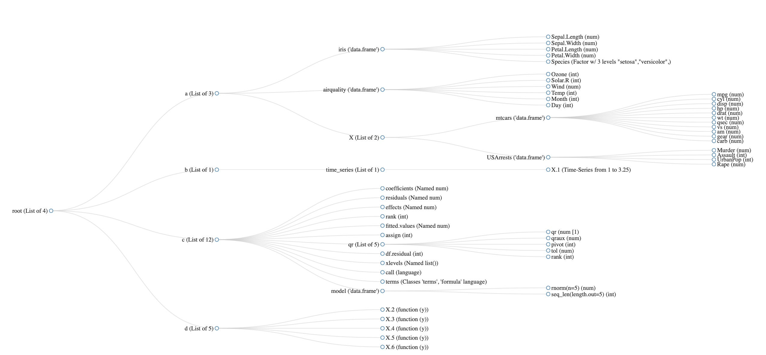
DataExplorer::plot_str()を用いるとnetworkD3パッケージを利用して、対象データセットの構造をネットワークグラフで可視化できます。
これによって、リストの入れ子で構造が複雑になったデータセットの把握がしやすくなります。ただし、シンプルな構造でネットワークグラフによる可視化が手間になるときなどは、先ほどのutils::str()やtibble::glimpse()を利用するのがよいでしょう。
nested_list %>% DataExplorer::plot_str(type = "diagonal", fontSize = 15)
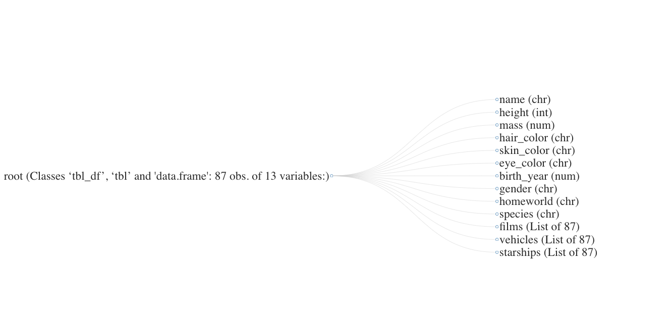
# 可視化するネストの深さの上限はmax_levelで指定
DataExplorer::plot_str(
  data = dplyr::starwars, type = "diagonal", max_level = 1,
  height = 600, width = 600, fontSize = 40
)
データセットの情報を可視化
データセットの可視化には様々な観点がありますが、この節で扱う関数は「データセット全体あるいは変数の決まった傾向の可視化」を対象にします(データセットを関数に渡して返ってくる結果を「探索」しない)。
引数で渡した変数で集計した傾向を見るケースや、データの散らばりや分布、変数間の関係性などを可視化する関数は次節にて触れます。
データセットの基本情報
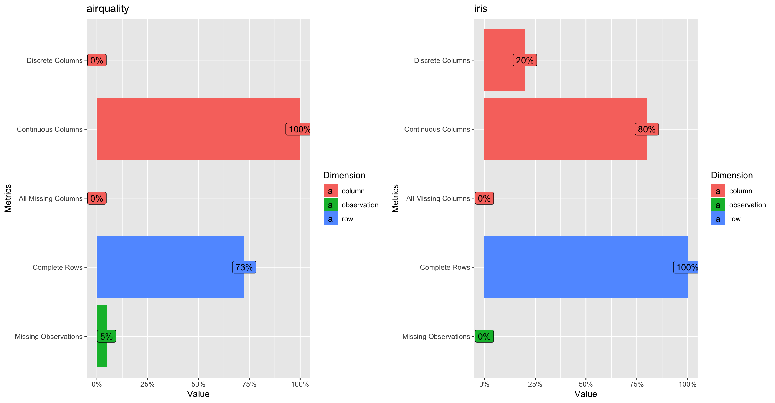
レコード・カラム数や離散・連続値のカラム数など、対象データセットの基本情報を算出する関数にDataExplorer::introduce()があり、DataExplorer::plot_intro()ではそれらの情報を可視化します。
ドキュメントには明示されていませんが、入力はデータフレームでなければならず、カラム中にはリストを含んでいてはいけません。
DataExplorer::introduce(data = datasets::iris) %>%
  tidyr::pivot_longer(
    cols = tidyselect::everything(), names_to = "var_name", values_to = "info"
  ) %>%
  dplyr::inner_join(
    # 結果の説明はドキュメントより
    y = tibble::tribble(
      ~var_name, ~desc,
      "rows", "number of rows",
      "columns", "number of columns",
      "discrete_columns", "number of discrete columns",
      "continuous_columns", "number of continuous columns",
      "all_missing_columns", "number of columns with everything missing",
      "total_missing_values", "number of missing observations",
      "complete_rows", "number of rows without missing values",
      "total_observations", "total number of observations",
      "memory_usage", "estimated memory allocation in bytes"
    ),
    by = c("var_name")
  )
# > # A tibble: 9 x 3
# >   var_name              info desc
# >   <chr>                <dbl> <chr>
# > 1 rows                   150 number of rows
# > 2 columns                  5 number of columns
# > 3 discrete_columns         1 number of discrete columns
# > 4 continuous_columns       4 number of continuous columns
# > 5 all_missing_columns      0 number of columns with everything missing
# > 6 total_missing_values     0 number of missing observations
# > 7 complete_rows          150 number of rows without missing values
# > 8 total_observations     750 total number of observations
# > 9 memory_usage          7976 estimated memory allocation in bytes

# 可視化
# Discrete Columns: discrete_columns / columns
# Continuous Columns: continuous_columns / columns
# All Missing Columns / columns
# Complete Rows: complete_rows / rows
# Missing Observations: missing_values / total_observations
pintro_iris <- DataExplorer::plot_intro(data = datasets::iris, title = "iris")
pintro_airq <- DataExplorer::plot_intro(data = datasets::airquality, title = "airquality")
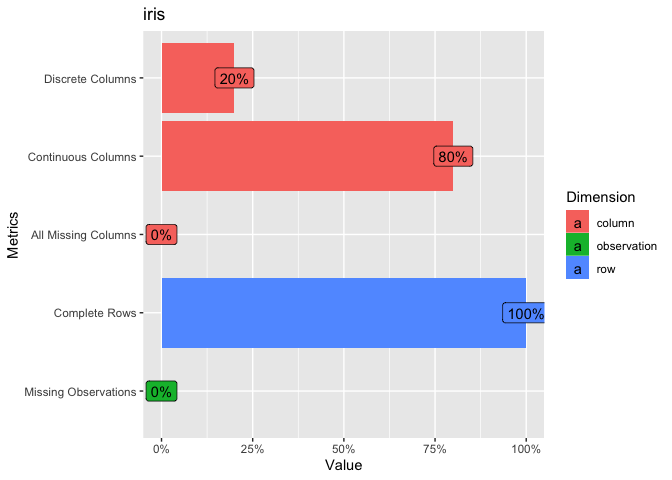
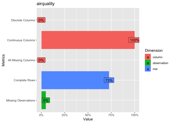
# それぞれの結果はggplotオブジェクトでpatchworkパッケージによる演算が可能
# patchworkパッケージがロード済みなら「+」で繋げるだけでよい
patchwork:::ggplot_add.ggplot(object = pintro_iris, plot = pintro_airq) +
  patchwork::plot_layout(ncol = 2)
# リストを含むデータセットはエラー
# DataExplorer::introduce(data = dplyr::starwars)
# > Error in complete.cases(data) : invalid 'type' (list) of argument

# 適用したい場合は対象カラムは取り除く必要がある
dplyr::starwars %>%
  dplyr::select_if(.predicate = purrr::negate(.p = is.list)) %>%
  # dplyr::select_if(.predicate = ~ !is.list(x = .x)) %>%
  DataExplorer:::introduce() %>%
  tidyr::pivot_longer(
    cols = tidyselect::everything(), names_to = "var_name", values_to = "info"
  )
# > # A tibble: 9 x 2
# >   var_name              info
# >   <chr>                <dbl>
# > 1 rows                    87
# > 2 columns                 10
# > 3 discrete_columns         7
# > 4 continuous_columns       3
# > 5 all_missing_columns      0
# > 6 total_missing_values   101
# > 7 complete_rows           29
# > 8 total_observations     870
# > 9 memory_usage         23960


data_explorer_funs_vari <- data_explorer_funs_vari %>%
  tibble::add_row(function_name = c("introduce", "plot_intro"))
データセットの欠損状況
DataExplorer::introduce()やDataExplorer::plot_intro()ではデータセット(対象はカラム中にリストを含まないデータフレーム)全体の欠損値数を計算・可視化できますが、どのカラムにどの程度欠損を含むかわかりません。
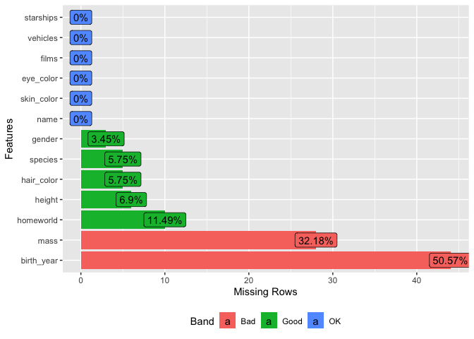
データセット中のカラム毎の欠損状況を個別に算出する関数にDataExplorer::profile_missing()があり、DataExplorer::plot_missing()ではそれらを可視化します。
これらの関数はカラム中にリストを含まないデータフレームにも対応しています。
# データセット中のカラム毎の欠損値情報
DataExplorer::profile_missing(data = dplyr::starwars) %>%
  # total_missingはDataExplorer:::introduceのtotal_missing_valuesと同じ値になる
  dplyr::add_tally(wt = num_missing, name = "total_missing")
# > # A tibble: 13 x 4
# >    feature    num_missing pct_missing total_missing
# >    <fct>            <int>       <dbl>         <int>
# >  1 name                 0      0                101
# >  2 height               6      0.0690           101
# >  3 mass                28      0.322            101
# >  4 hair_color           5      0.0575           101
# >  5 skin_color           0      0                101
# >  6 eye_color            0      0                101
# >  7 birth_year          44      0.506            101
# >  8 gender               3      0.0345           101
# >  9 homeworld           10      0.115            101
# > 10 species              5      0.0575           101
# > 11 films                0      0                101
# > 12 vehicles             0      0                101
# > 13 starships            0      0                101
# 計算検証
dplyr::starwars %>% is.na() %>% colSums() %>%
  tibble::enframe(name = "feature", value = "num_missing") %>%
  # pct_missingは「num_missing / データセットのレコード数」
  dplyr::mutate(pct_missing = num_missing / (dplyr::starwars %>% nrow()))
# > # A tibble: 13 x 3
# >    feature    num_missing pct_missing
# >    <chr>            <dbl>       <dbl>
# >  1 name                 0      0
# >  2 height               6      0.0690
# >  3 mass                28      0.322
# >  4 hair_color           5      0.0575
# >  5 skin_color           0      0
# >  6 eye_color            0      0
# >  7 birth_year          44      0.506
# >  8 gender               3      0.0345
# >  9 homeworld           10      0.115
# > 10 species              5      0.0575
# > 11 films                0      0
# > 12 vehicles             0      0
# > 13 starships            0      0

# カラム毎の欠損比率を可視化
dplyr::starwars %>%
  DataExplorer::plot_missing(
    # group引数でグループ分けと比率の上限値を定義できる
    group = list("OK" = 0.00, "Good" = 0.20, "Bad" = 0.99, "Remove" = 1.00)
  )


data_explorer_funs_vari <- data_explorer_funs_vari %>%
  tibble::add_row(function_name = c("profile_missing", "plot_missing"))
データセット中にある変数の情報を可視化
統計モデリングや予測モデル構築などを始めるにあたって、変数の分布や関係性などを可視化してデータの理解を深めてから行います。
DataExplorerパッケージはggplot2パッケージをラップする形で基本的な可視化用関数を提供しています。
関数名に対応する可視化方法(plot_barは棒グラフ、plot_boxplotは箱ひげ図など)で、当てはめたデータセットが持つ「連続変数・離散変数、または指定カラムに応じて可視化」されます。説明だけでは理解しづらいですので、関数毎にデータを可視化して挙動を確認します。
plot_bar
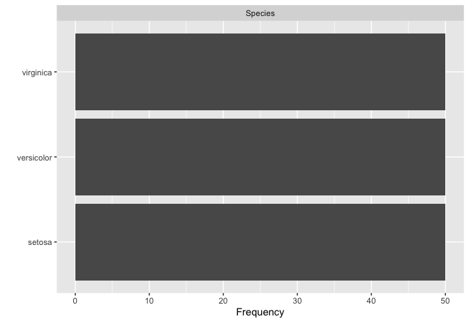
DataExplorer::plot_bar()は離散変数カラム別・離散変数値毎に集計した結果を棒グラフで可視化します。
変数の傾向をざっと掴むという観点では前節の関数群に該当しそうですが、with引数によって対象を探索的に見られるという点でこちらで説明しています。
DataExplorer::plot_bar(data = datasets::iris)
# 以下の集計結果を可視化すると同じになる
datasets::iris %>% dplyr::group_by(Species) %>% dplyr::tally()
# > # A tibble: 3 x 2
# >   Species        n
# >   <fct>      <int>
# > 1 setosa        50
# > 2 versicolor    50
# > 3 virginica     50
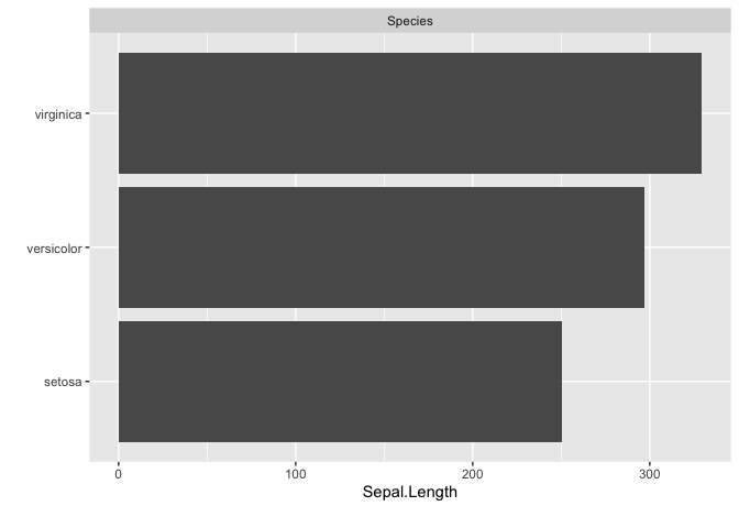
# with引数で指定した連続値を集計
DataExplorer::plot_bar(data = datasets::iris, with = "Sepal.Length")
# 以下の集計結果を可視化すると同じになる
datasets::iris %>% dplyr::group_by(Species) %>% dplyr::tally(wt = Sepal.Length)
# > # A tibble: 3 x 2
# >   Species        n
# >   <fct>      <dbl>
# > 1 setosa      250.
# > 2 versicolor  297.
# > 3 virginica   329.
# 複数離散変数カラムがあるデータは離散変数カラムで分けられ(ggplot2::facet_wrap)、属するカラムの離散変数値をy軸に取ってプロット
DataExplorer::plot_bar(data = ggplot2::diamonds, with = "price")
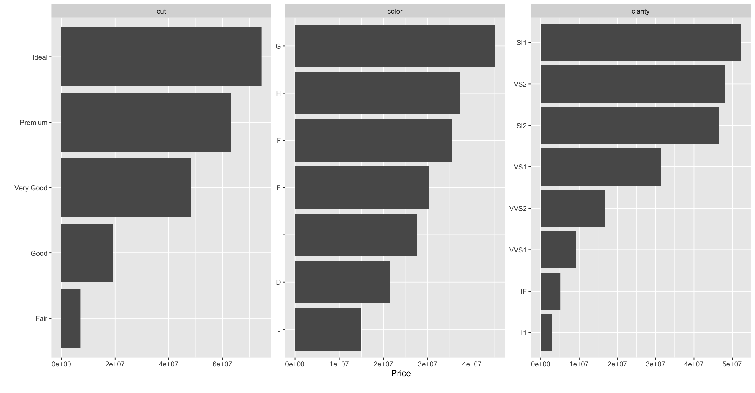
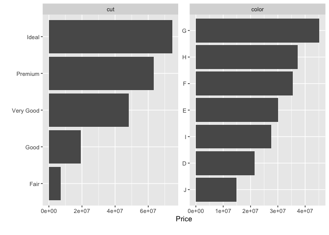
# maxcat引数で指定した値より多い種類数がある離散変数カラムを除外
DataExplorer::plot_bar(data = ggplot2::diamonds, with = "price", maxcat = 7)
# > 1 columns ignored with more than 7 categories.
# > clarity: 8 categories


data_explorer_funs_vari <- data_explorer_funs_vari %>%
  tibble::add_row(function_name = c("plot_bar"))
plot_scatterplot/boxplot/density/histogram
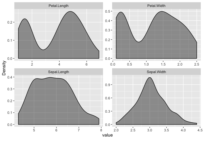
データの分布や形状を把握するには散布図や箱ひげ図などの可視化方法がありますが、これらに対応したDataExplorer::plot_scatterplot(), DataExplorer::plot_boxplot(), DataExplorer::plot_density(), DataExplorer::plot_histogram()がDataExplorerパッケージでは提供されています。
データセットをそれぞれの関数に適用すると、次のような可視化結果が得られます。
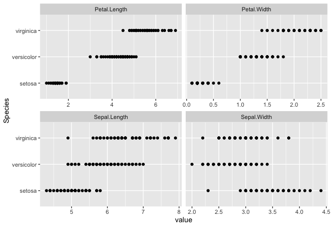
DataExplorer::plot_scatterplot(
  data = datasets::iris, by = "Species", nrow = 2, ncol = 2
)
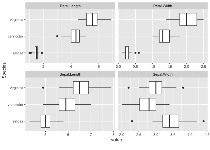
DataExplorer::plot_boxplot(
  data = datasets::iris, by = "Species", nrow = 2, ncol = 2
)
DataExplorer::plot_density(
  data = datasets::iris, nrow = 2, ncol = 2,
  geom_density_args = list("fill" = "black", "alpha" = 0.4)
)
DataExplorer::plot_histogram(
  data = datasets::iris, nrow = 2, ncol = 2,
  geom_histogram_args = list("bins" = 30, "fill" = "black", "alpha" = 0.4)
)

data_explorer_funs_vari <- data_explorer_funs_vari %>%
  tibble::add_row(
    function_name = c(
      "plot_scatterplot", "plot_boxplot", "plot_density", "plot_histogram"
    )
  )
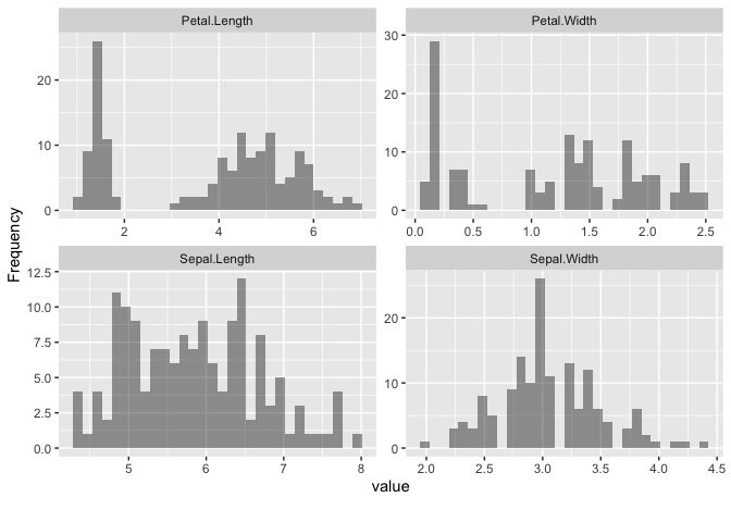
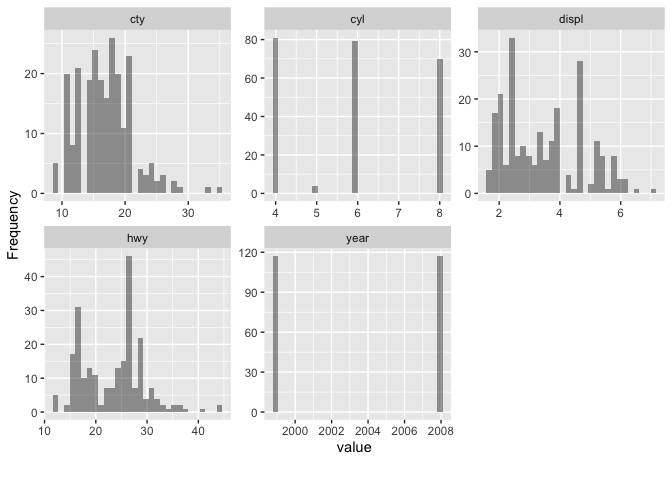
DataExplorer::plot_density()とDataExplorer::plot_histogram()は連続値を持つカラムのみを対象に、よしなに可視化してくれます。
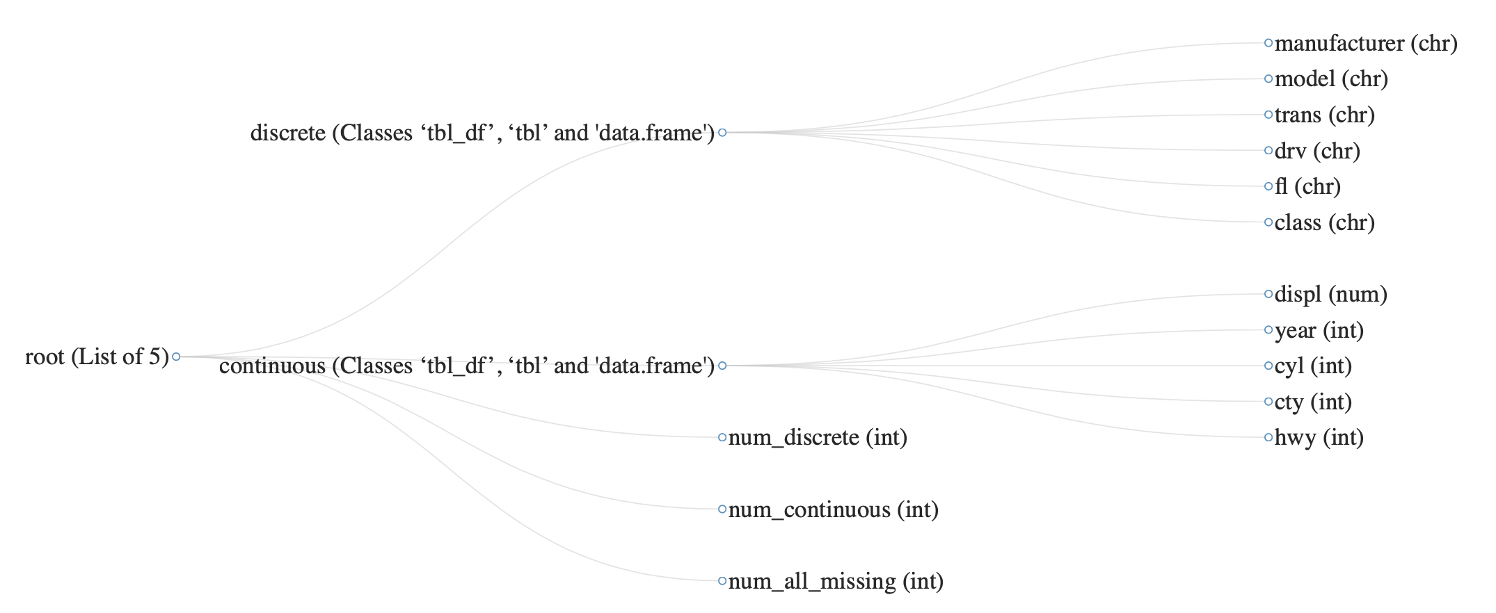
このときDataExplorer::split_columns()が関数内部で呼ばれており、この関数は入力したデータセットを離散変数カラムのデータフレームと連続変数カラムのデータフレームに分けてくれます。
# 数値からなるデータフレームと、文字列からなるデータフレームに分かれ
# num_*でそれらの情報を表す数値が含まれている
DataExplorer::plot_str(
  data = DataExplorer::split_columns(data = ggplot2::mpg),
  height = 800, width = 1400, fontSize = 30
)
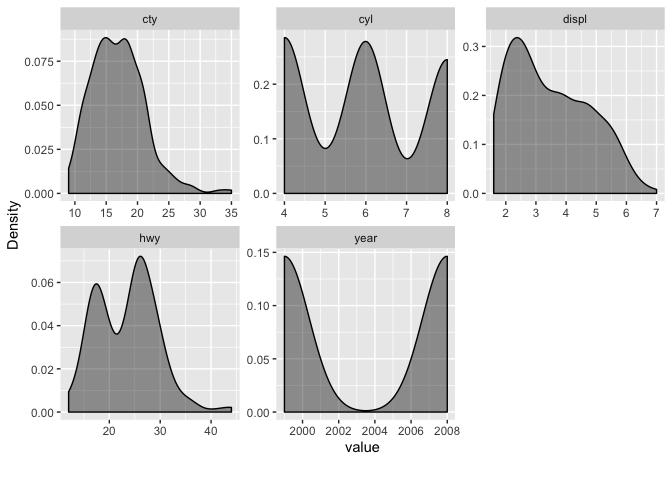
# 連続変数カラム名
DataExplorer::split_columns(data = ggplot2::mpg)$continuous %>%
  colnames() %>% print()
# > [1] "displ" "year"  "cyl"   "cty"   "hwy"

# 対象カラムを可視化
DataExplorer::plot_density(
  data = ggplot2::mpg, nrow = 2, ncol = 3,
  # 2種類要素の整数値カラムがバイナリ扱いにされるため、FALSEを指定して避ける
  binary_as_factor = FALSE,
  geom_density_args = list("fill" = "black", "alpha" = 0.4)
)
DataExplorer::plot_histogram(
  data = ggplot2::mpg, nrow = 2, ncol = 3,
  binary_as_factor = FALSE,
  geom_histogram_args = list("bins" = 30, "fill" = "black", "alpha" = 0.4)
)


data_explorer_funs_vari <- data_explorer_funs_vari %>%
  tibble::add_row(function_name = c("split_columns"))
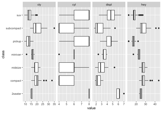
DataExplorer::plot_boxplot()も連続値を持つカラムが可視化対象ですが、DataExplorer::plot_scatterplot()は両方ともが対象です。
両関数ともにby引数でy軸に設定するカラム名を1種類まで指定できますが、DataExplorer::plot_boxplot()は連続変数のカラム名を指定すると数値区間を同分割(5分割)して離散化します。
# 離散変数カラム名
DataExplorer::split_columns(data = ggplot2::mpg)$discrete %>%
  colnames() %>% print()
# > [1] "manufacturer" "model"        "trans"        "drv"
# > [5] "fl"           "class"

# by引数の複数個指定はできない
# DataExplorer::plot_boxplot(data = ggplot2::mpg, by = c("class", "manufacturer"))

DataExplorer::plot_boxplot(
  # ggplot2::mpgのyearは「1999と2008」の2種類しかなく可視化対象に含めない
  data = ggplot2::mpg, by = "class", ncol = 4, binary_as_factor = TRUE
)
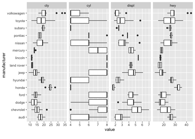
DataExplorer::plot_boxplot(
  # ggplot2::mpgのyearは「1999と2008」の2種類しかなく可視化対象に含めない
  data = ggplot2::mpg, by = "manufacturer", ncol = 4, binary_as_factor = TRUE
)
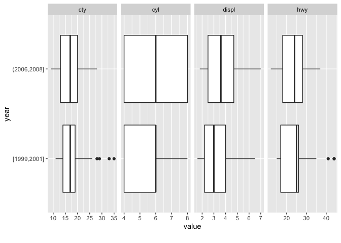
# by引数で指定した連続変数を離散化
# 「1999と2008」の2種類
ggplot2::cut_interval(x = ggplot2::mpg$year, n = 5) %>%
  forcats::fct_drop() %>% levels()
# > [1] "[1999,2001]" "(2006,2008]"
DataExplorer::plot_boxplot(data = ggplot2::mpg, by = "year", ncol = 4)
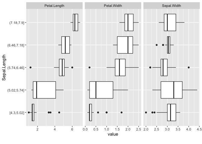
ggplot2::cut_interval(x = datasets::iris$Sepal.Length, n = 5) %>%
  forcats::fct_drop() %>% levels()
# > [1] "[4.3,5.02]"  "(5.02,5.74]" "(5.74,6.46]" "(6.46,7.18]" "(7.18,7.9]"
DataExplorer::plot_boxplot(data = datasets::iris, by = "Sepal.Length", ncol = 4)
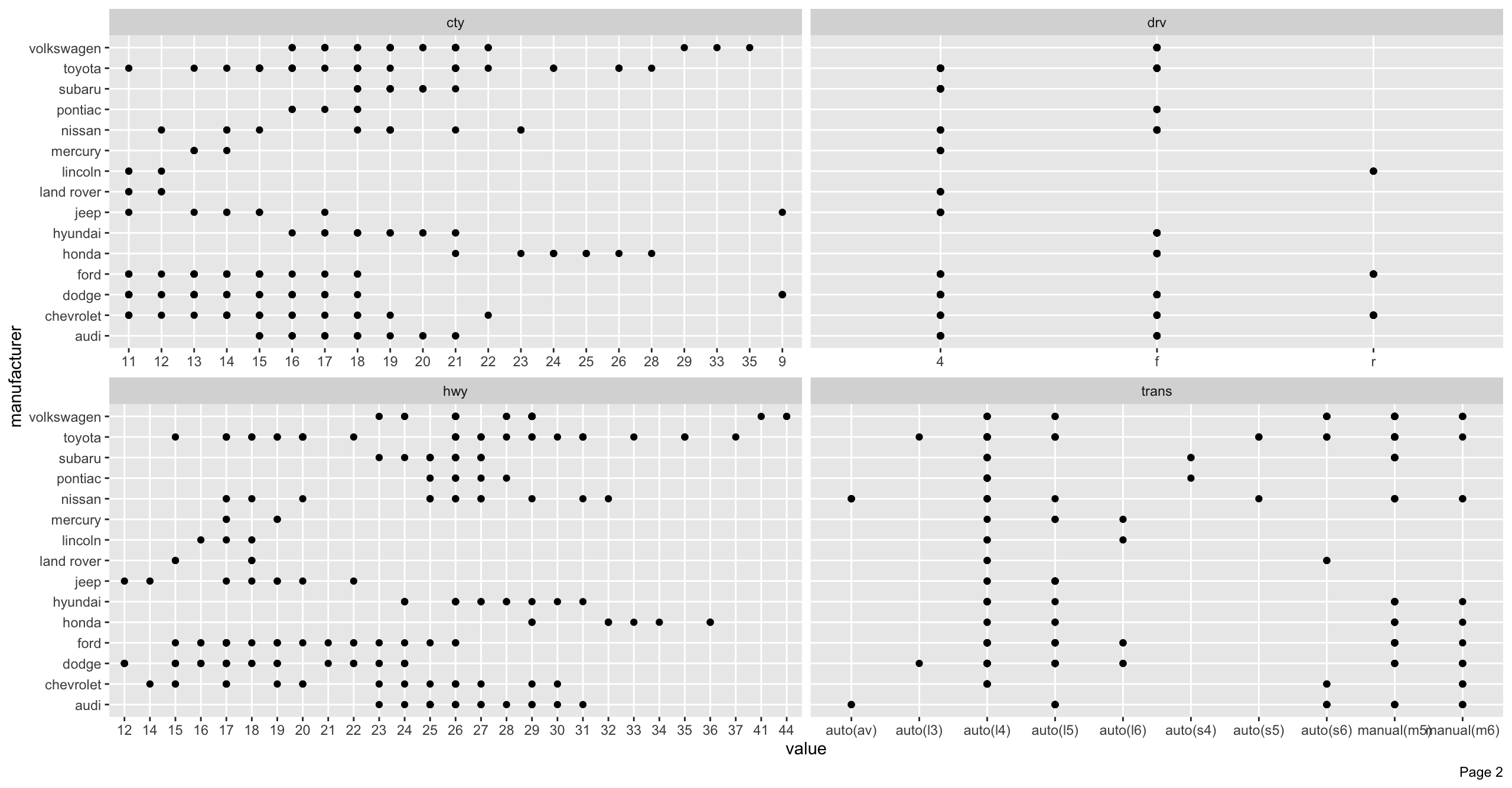
manufacturer_scatterplot <- DataExplorer::plot_scatterplot(
  data = ggplot2::mpg, by = "manufacturer", nrow = 2, ncol = 2
)
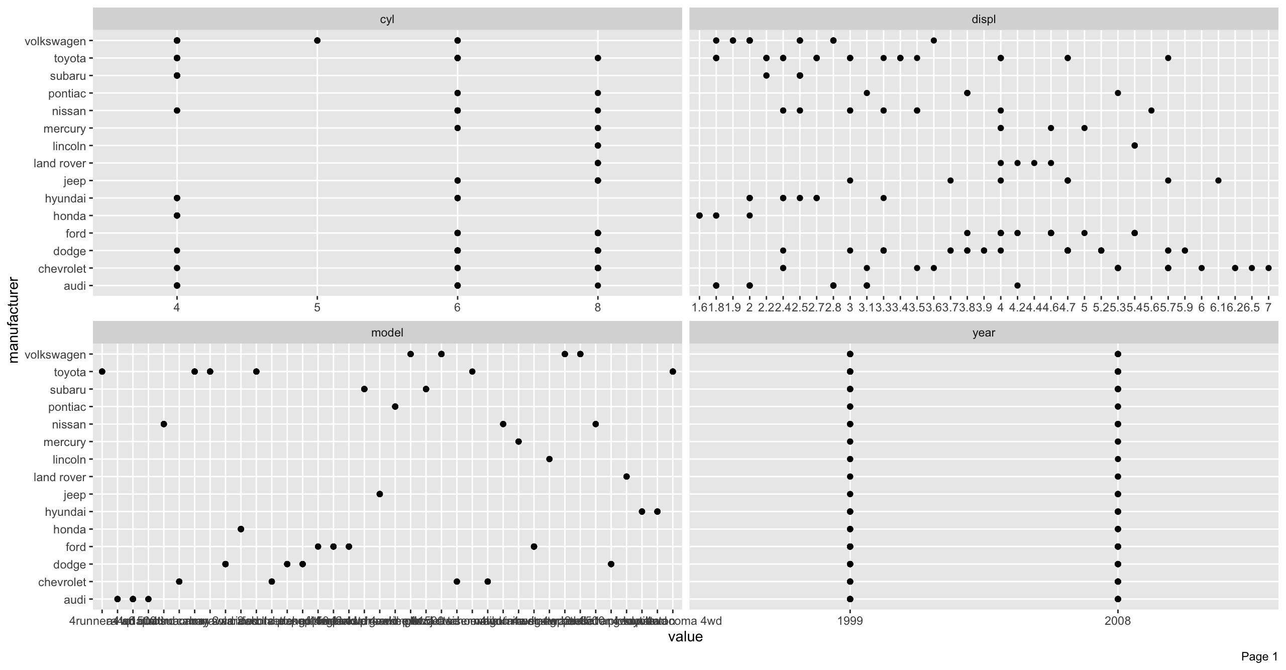
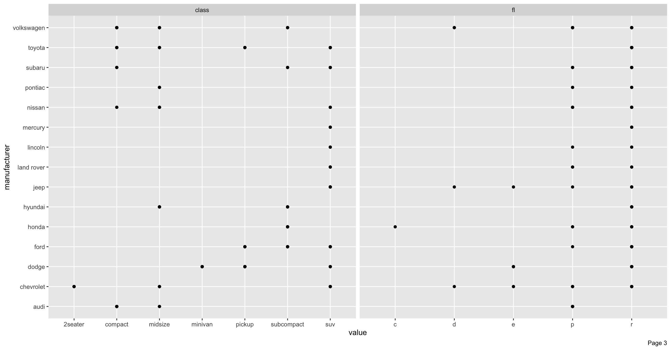
# 可視化領域を越えた場合はページングが発生して結果のリスト中にある「page_*」で取り出せる
print(x = names(x = manufacturer_scatterplot))
# > [1] "page_1" "page_2" "page_3"
# Page 2の可視化結果を再度表示
print(manufacturer_scatterplot$page_2)

plot_correlation/prcomp/qq
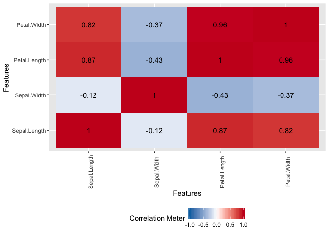
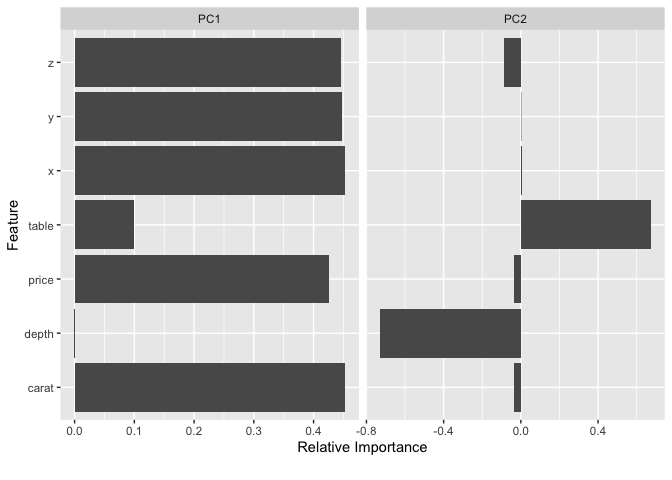
DataExplorerパッケージでは、上記の他に「変数間の相関係数をヒートマップの形で可視化」するDataExplorer::plot_correlation()や「主成分分析による結果を主成分毎に可視化(指定した寄与率の累積まで)」するDataExplorer::plot_prcomp()に「連続変数毎のQ-Qプロット」を出すDataExplorer::plot_qq()も定義されています。
# plot_correlation
# type = "continuous" or "c"は算出対象を連続変数に限定
DataExplorer::plot_correlation(data = datasets::iris, type = "continuous")
# 可視化される結果と同じ数値になる
DataExplorer::split_columns(data = datasets::iris)$continuous %>%
  cor() %>% round(digits = 2)
# >              Sepal.Length Sepal.Width Petal.Length Petal.Width
# > Sepal.Length         1.00       -0.12         0.87        0.82
# > Sepal.Width         -0.12        1.00        -0.43       -0.37
# > Petal.Length         0.87       -0.43         1.00        0.96
# > Petal.Width          0.82       -0.37         0.96        1.00
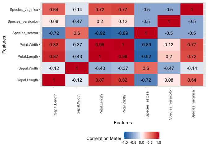
# 離散変数はダミー変数化して算出&可視化
DataExplorer::plot_correlation(data = datasets::iris, type = "all")
# 相関係数の計算にはstats::corが用いられるため欠損値が含まれる場合はcor_args引数で扱いを指定する
DataExplorer::plot_correlation(data = datasets::airquality, type = "all")
# > Warning: Removed 18 rows containing missing values (geom_text).
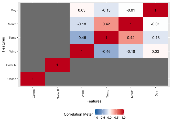
# 欠損値処理をして可視化
DataExplorer::plot_correlation(
  data = datasets::airquality, type = "all",
  cor_args = list("use" = "pairwise.complete.obs")
)

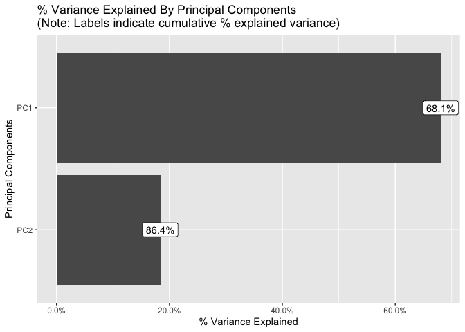
# plot_prcomp
PCA_VARIANCE_CAP <- 0.9 # 寄与率累積の閾値
DataExplorer::plot_prcomp(
  data = DataExplorer::split_columns(data = ggplot2::diamonds)$continuous,
  variance_cap = PCA_VARIANCE_CAP, prcomp_args = list(scale. = TRUE),
  ncol = 2, nrow = 2
)
# 可視化結果と同じになる数値を出す
result_pca <- prcomp(
  x = DataExplorer::split_columns(data = ggplot2::diamonds)$continuous,
  scale. = TRUE
)
# broom:::tidy.prcomp
result_pca %>%
  broom::tidy(matrix = "rotation") %>%
  dplyr::mutate(
    PC = stringr::str_c("PC", .$PC),
    value = round(x = .$value, digits = 2)
  ) %>%
  tidyr::pivot_wider(names_from = "PC", values_from = "value") %>% print()
# > # A tibble: 7 x 8
# >   column   PC1   PC2   PC3   PC4   PC5   PC6   PC7
# >   <chr>  <dbl> <dbl> <dbl> <dbl> <dbl> <dbl> <dbl>
# > 1 carat   0.45 -0.03  0.01 -0.07  0.13  0.77  0.43
# > 2 depth   0    -0.73 -0.67 -0.05 -0.09  0.01 -0.06
# > 3 table   0.1   0.68 -0.73 -0.06 -0.01 -0.03  0
# > 4 price   0.43 -0.04  0.11 -0.85 -0.05 -0.27 -0.08
# > 5 x       0.45  0     0.04  0.24  0.09  0.2  -0.83
# > 6 y       0.45  0     0.05  0.33 -0.77 -0.22  0.21
# > 7 z       0.45 -0.09 -0.04  0.32  0.6  -0.5   0.28
result_pca %>%
  broom::tidy(matrix = "d") %>%
  dplyr::mutate(PC = stringr::str_c("PC", .$PC)) %>%
  # 閾値判定
  # DataExplorer::plot_prcompではvariance_cap引数の値までを可視化
  dplyr::mutate(cumulative <= PCA_VARIANCE_CAP) %>% print()
# > # A tibble: 7 x 5
# >   PC    std.dev percent cumulative `cumulative <= PCA_VARIANCE_CAP`
# >   <chr>   <dbl>   <dbl>      <dbl> <lgl>
# > 1 PC1     2.18  0.681        0.681 TRUE
# > 2 PC2     1.13  0.184        0.864 TRUE
# > 3 PC3     0.831 0.0987       0.963 FALSE
# > 4 PC4     0.417 0.0248       0.988 FALSE
# > 5 PC5     0.201 0.00576      0.994 FALSE
# > 6 PC6     0.182 0.00471      0.998 FALSE
# > 7 PC7     0.111 0.00177      1     FALSE
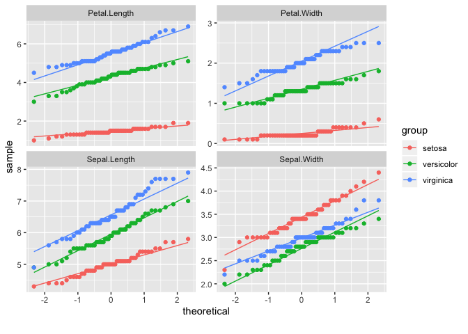
# plot_qq
# Q-Qプロットはデータが「ある確率分布に従っているかどうか」を調査する際に使われる
# ほぼ直線上に散布図の点が並んでいればデータはその確率分布に従っていると考えられる
# 調査対象の確率分布はgeom_qq_args引数とgeom_qq_line_args引数で指定可能(ggplot2::geom_qq/geom_qq_lineに設定が渡される)
# by引数はDataExplorer::plot_boxplot同様
DataExplorer::plot_qq(data = datasets::iris, by = "Species", nrow = 2, ncol = 2)
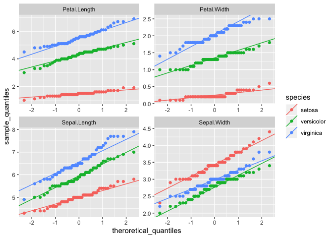
# 可視化結果と同じになる数値を出す関数
pointQQxy <- function(...) {
  computeSlopeIntercept <- function(...) {
    arg_list <- rlang::list2(...)
    x <- qnorm(p = c(0.25, 0.75))
    y <- quantile(
      x = arg_list[[1]] %>% dplyr::pull(), probs = c(0.25, 0.75),
      names = FALSE, na.rm = TRUE
    )
    tibble::tibble(
      var = arg_list[[2]]$var,
      slope = diff(y) / diff(x), intercept = y[1L] - (slope * x[1L])
    ) %>%
      dplyr::bind_rows() %>%
      return()
  }

  arg_list <- rlang::list2(...)
  s_quantile <- arg_list[[1]] %>%
    tidyr::pivot_longer(
      cols = tidyselect::everything(),
      names_to = "var", values_to = "sample_quantiles"
    ) %>%
    dplyr::group_by(var)

  s_quantile %>%
    dplyr::arrange(sample_quantiles) %>% dplyr::add_tally() %>%
    dplyr::mutate(theroretical_quantiles = qnorm(p = ppoints(n = n))) %>%
    dplyr::left_join(
      y = s_quantile %>%
        dplyr::group_map(.f = computeSlopeIntercept) %>% dplyr::bind_rows(),
      by = c("var")
    ) %>%
    dplyr::select(-n) %>%
    dplyr::mutate(species = arg_list[[2]]$Species) %>%
    return()
}

datasets::iris %>%
  dplyr::group_by(Species) %>%
  dplyr::group_map(.f = pointQQxy, keep = FALSE) %>% dplyr::bind_rows() %>%
  ggplot2::ggplot() +
  ggplot2::geom_point(
    mapping = ggplot2::aes(
      x = theroretical_quantiles, y = sample_quantiles, colour = species
    )
  ) +
  ggplot2::geom_abline(
    mapping = ggplot2::aes(slope = slope, intercept = intercept, colour = species)
  ) +
  ggplot2::facet_wrap(facets = ~var, nrow = 2, ncol = 2, scales = "free")
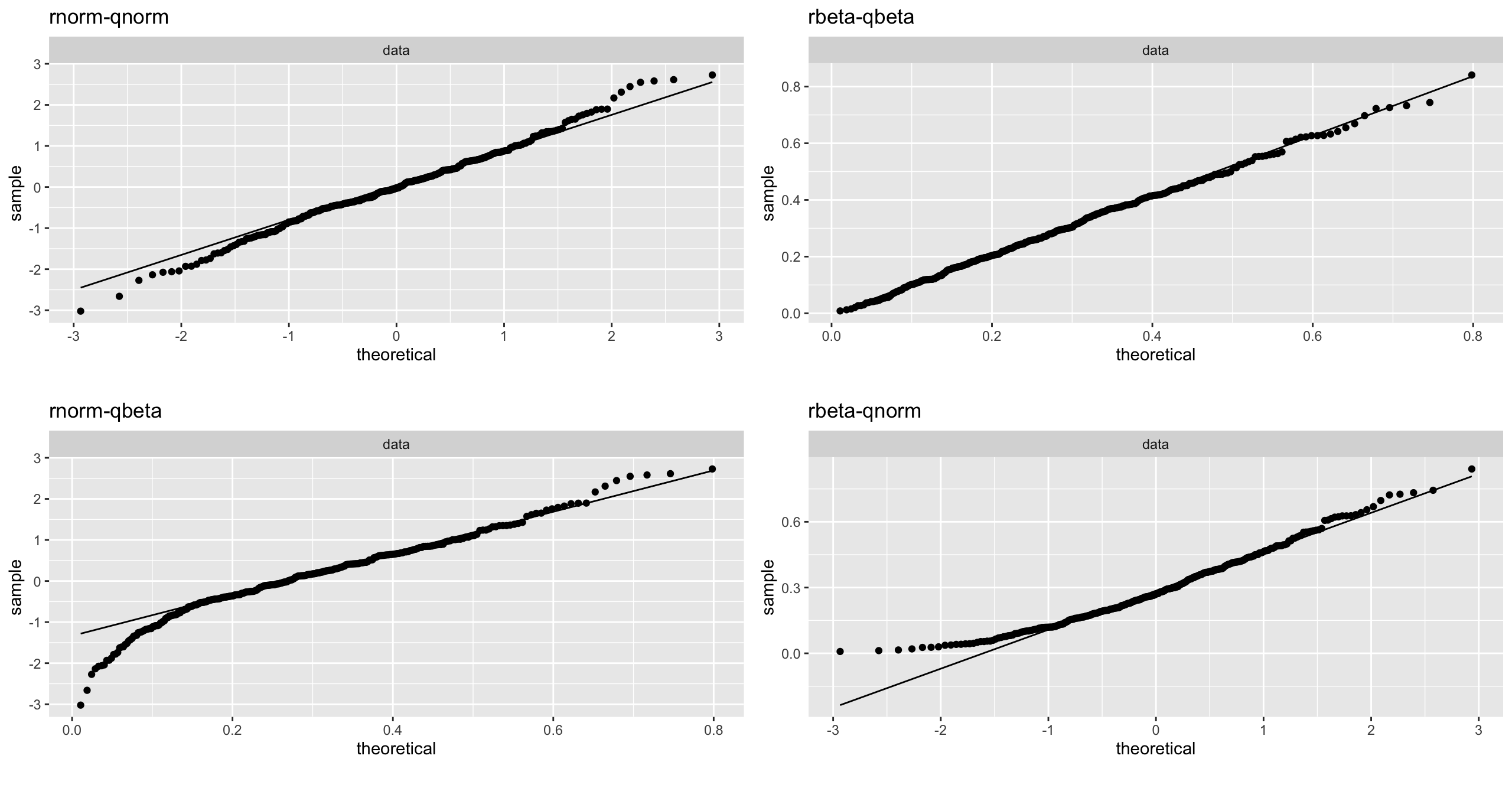
# 疑似データでQQプロットを試す
set.seed(seed = 100)
smpl_dst <- tibble::tibble(
  # 正規分布に従う乱数
  norm = rnorm(n = 300, mean = 0, sd = 1),
  # ベータ分布に従う乱数
  beta = rbeta(n = 300, shape1 = 2, shape2 = 5)
)
smpl_args <- tibble::lst(
  norm = tibble::lst(
    distribution = stats::qnorm, dparams = list(mean = 0, sd = 1)
  ),
  beta = tibble::lst(
    distribution = stats::qbeta, dparams = list(shape1 = 2, shape2 = 5)
  )
)

# それぞれをQQプロットで可視化
qq_facet <- (
  DataExplorer::plot_qq(
    # 正規分布に従う乱数で正規分布検証
    data = smpl_dst$norm, title = "rnorm-qnorm",
    geom_qq_args = smpl_args$norm, geom_qq_line_args = smpl_args$norm
  )$page_1 +
  DataExplorer::plot_qq(
    # ベータ分布に従う乱数でベータ分布検証
    data = smpl_dst$beta, title = "rbeta-qbeta",
    geom_qq_args = smpl_args$beta, geom_qq_line_args = smpl_args$beta
  )$page_1 +
  DataExplorer::plot_qq(
    # 正規分布に従う乱数でベータ分布検証
    data = smpl_dst$norm, title = "rnorm-qbeta",
    geom_qq_args = smpl_args$beta, geom_qq_line_args = smpl_args$beta
  )$page_1 +
  DataExplorer::plot_qq(
    # ベータ分布に従う乱数で正規分布検証
    data = smpl_dst$beta, title = "rbeta-qnorm",
    geom_qq_args = smpl_args$norm, geom_qq_line_args = smpl_args$norm
  )$page_1
)
# 乱数生成と検証対象の分布が同じである上は直線とのずれが少ないが、それらが異なる下は乖離が見られる
qq_facet + patchwork::plot_layout(ncol = 2)


data_explorer_funs_vari <- data_explorer_funs_vari %>%
  tibble::add_row(
    function_name = c("plot_correlation", "plot_prcomp", "plot_qq")
  )
特徴量エンジニアリング
DataExplorerパッケージには可視化だけでなく特徴量エンジニアリングに役立てられる関数も定義されていますので、簡単に紹介しておきます。
DataExplorer::dummify()はダミー変数作成の関数です。recipes/caret/mlr/dummyなどのパッケージでも行えますが、与えるデータ形式と使い方に応じて選ぶと良いと思います。
DataExplorer::group_category()は離散変数中にある、低頻度要素をひとつにまとめる関数です。値が低い順から指定した閾値までの要素が集約されます。
# dummify
datasets::iris %>%
  dplyr::group_by(Species) %>%
  dplyr::group_map(.f = head, n = 3, keep = TRUE) %>%
  dplyr::bind_rows() %>%
  # selectで選んだ変数をダミー変数化(連続変数は無視される)
  DataExplorer::dummify(select = "Species")
# > # A tibble: 9 x 7
# >   Sepal.Length Sepal.Width Petal.Length Petal.Width Species_setosa
# >          <dbl>       <dbl>        <dbl>       <dbl>          <int>
# > 1          5.1         3.5          1.4         0.2              1
# > 2          4.9         3            1.4         0.2              1
# > 3          4.7         3.2          1.3         0.2              1
# > 4          7           3.2          4.7         1.4              0
# > 5          6.4         3.2          4.5         1.5              0
# > 6          6.9         3.1          4.9         1.5              0
# > 7          6.3         3.3          6           2.5              0
# > 8          5.8         2.7          5.1         1.9              0
# > 9          7.1         3            5.9         2.1              0
# > # … with 2 more variables: Species_versicolor <int>,
# > #   Species_virginica <int>


# group_category
mpg_mmc <- ggplot2::mpg %>%
  dplyr::select(manufacturer, model, class)
mpg_mmc %>%
  dplyr::group_by(class) %>%
  dplyr::tally() %>%
  dplyr::arrange(dplyr::desc(x = n))
# > # A tibble: 7 x 2
# >   class          n
# >   <chr>      <int>
# > 1 suv           62
# > 2 compact       47
# > 3 midsize       41
# > 4 subcompact    35
# > 5 pickup        33
# > 6 minivan       11
# > 7 2seater        5

# 「update = FALSE」のときは閾値(threshold引数)に応じた集計情報を表示
# 「threshold = 0」はまとめない
mpg_mmc %>%
  DataExplorer::group_category(feature = "class", threshold = 0.00) %>%
  # 「cum_pct <= (1 - threshold)」がまとめらる
  dplyr::mutate(1 - cum_pct)
# > # A tibble: 7 x 5
# >   class        cnt    pct cum_pct `1 - cum_pct`
# >   <chr>      <int>  <dbl>   <dbl>         <dbl>
# > 1 suv           62 0.265    0.265        0.735
# > 2 compact       47 0.201    0.466        0.534
# > 3 midsize       41 0.175    0.641        0.359
# > 4 subcompact    35 0.150    0.791        0.209
# > 5 pickup        33 0.141    0.932        0.0684
# > 6 minivan       11 0.0470   0.979        0.0214
# > 7 2seater        5 0.0214   1            0
mpg_mmc %>%
  # 「class = "pickup"」はそのまま
  DataExplorer::group_category(feature = "class", threshold = 0.0683)
# > # A tibble: 5 x 4
# >   class        cnt   pct cum_pct
# >   <chr>      <int> <dbl>   <dbl>
# > 1 suv           62 0.265   0.265
# > 2 compact       47 0.201   0.466
# > 3 midsize       41 0.175   0.641
# > 4 subcompact    35 0.150   0.791
# > 5 pickup        33 0.141   0.932
mpg_mmc %>%
  # 「class = "pickup"」はまとめる
  DataExplorer::group_category(feature = "class", threshold = 0.0684)
# > # A tibble: 4 x 4
# >   class        cnt   pct cum_pct
# >   <chr>      <int> <dbl>   <dbl>
# > 1 suv           62 0.265   0.265
# > 2 compact       47 0.201   0.466
# > 3 midsize       41 0.175   0.641
# > 4 subcompact    35 0.150   0.791

# 「update = TRUE」で離散変数値を集約
# category_name引数に指定した名称がつけられる
mpg_mmc %>%
  DataExplorer::group_category(
    feature = "class", threshold = 0.0684,
    category_name = "OTHER", update = TRUE
  ) %>%
  dplyr::group_by(class) %>% dplyr::tally() %>%
  dplyr::arrange(dplyr::desc(x = n))
# > # A tibble: 5 x 2
# >   class          n
# >   <chr>      <int>
# > 1 suv           62
# > 2 OTHER         49
# > 3 compact       47
# > 4 midsize       41
# > 5 subcompact    35
飛ばした関数
本記事で割愛した関数には以下があります。
DataExplorer::create_report()は、config引数またはDataExplorer::configure_report()で設定した内容に従って、本記事で解説したDataExplorerパッケージで定義されている関数群を用いた可視化をまとめたHTMLファイルを生成します。
ここでは詳しく解説していませんが、DataExplorerパッケージの価値はこの関数にあると言っても過言ではありません。
DataExplorer::plotDataExplorer()はDataExplorerパッケージの各種可視化関数内で呼び出されるggplot2パッケージのラッパー関数になります。
DataExplorer::drop_columns()はdplyr::select(), DataExplorer::update_columns()はdplyr::mutate(), DataExplorer::set_missing()はtidyr::replace_na()の機能におおよそ相当する関数です。
DataExplorerパッケージの作者はdata.tableパッケージを好んで使っているようで、dplyr/tidyrは出てきません。
data_explorer_functions %>%
  dplyr::filter(ns == "DataExplorer") %>%
  dplyr::anti_join(y = data_explorer_funs_vari, by = "function_name") %>% print(n = Inf)
# > # A tibble: 6 x 2
# >   function_name    ns
# >   <chr>            <chr>
# > 1 configure_report DataExplorer
# > 2 create_report    DataExplorer
# > 3 drop_columns     DataExplorer
# > 4 plotDataExplorer DataExplorer
# > 5 set_missing      DataExplorer
# > 6 update_columns   DataExplorer
まとめ
DataExplorerパッケージについて、実際に動作を確認しながら機能を解説しました。
データセットを様々な観点で可視化して探索的データ解析の効率を上げるだけでなく、例えば日次更新テーブルを日別で可視化して状態をざっと把握するなどの基盤運用にも利用できそうですね。
このようなデータセットの統計情報を算出・可視化するパッケージには、他にも以下のようなものがあります。
- skimr: Compact and Flexible Summaries of Data (CRAN)
- summarytools: Tools to Quickly and Neatly Summarize Data
- inspectdf: Inspection, Comparison and Visualisation of Data Frames
skimr/summarytoolsパッケージにはありますが、base::summary()で得られるデータセットの統計情報を算出する関数はDataExplorerパッケージには今のところなく、これらのパッケージ群との機能比較や組み合わせた使い方も興味深いところです。
ちなみにPythonではpandas-profilingで似たことが実現できるそうです。
DataExplorerパッケージはデータセットの可視化を手軽にして、データ理解にかける時間を抑えて探索的データ解析を手助けしてくれますが、もっと手軽に探索的データ解析をするアプローチもあります。やりたいこととスキルセットに応じてこれらを合わせて使うのも良いでしょう。
参考
- R for Data Science - 7 Exploratory Data Analysis
- edarf パッケージ:ランダムフォレストで探索的データ分析
- DataWrangling ~Exploratory Data Analysis:diamonds~
- DASKによる探索的データ分析(EDA)
- Radiantによるデータ分析入門
- patchworkを使って複数のggplotを組み合わせる
- 主成分分析の考え方
- データ解析その前に: 分布型の確認と正規性の検定
- 【統計学】Q-Qプロットの仕組みをアニメーションで理解する。
- 63. 正規性の検定
- Normal Q-Q プロットを理解する
- qqnorm and qqline in ggplot2
- 離散値化
- 連続値データの離散化(R Advent Calendar 2013)
余談
2013年くらいにGartner社が開催した「Business Intelligence & Analytics Summit」で触れられていたという話を読んで私は知りましたが(Web上にはっきりとした資料は見つけられませんでした)、データ分析は次の4ステップからなるそうです。
- Descriptive Analytics: 記述的分析(何が起きたのか?)
- Diagnostic Analytics: 診断的分析(なぜ起こったのか?)
- Predictive Analytics: 予測的分析(何が起きるのか?)
- Prescriptive Analytics: 処方的分析(何をすべきか?)
「Descriptive Diagnostic Predictive Prescriptive Analytics」で画像検索すると矢印が右上に向かった図が出てきますし、NECの特集コンテンツのページには別開催時の講演解説があります。他にも以下のようなページは数多く見つかります。
- The Four Types of Data Analytics
- 5 Types of analytics: Prescriptive, Predictive, Diagnostic, Descriptive and Cognitive Analytics
データを可視化して「何がどこで起きているかを知る・気づく」フェーズはBIツールの導入によって普及してきましたが、データからインサイトを得て「なぜ起きたか説明できる」フェーズは手軽ではなく広がっているとは言えず、探索的データ解析の自動化はひとつのアプローチと考えられます。
実行環境
sessioninfo::session_info()
─ Session info ─────────────────────────────────────────────────
 setting  value
 version  R version 3.5.1 (2018-07-02)
 os       macOS  10.14.4
 system   x86_64, darwin15.6.0
 ui       RStudio
 language (EN)
 collate  ja_JP.UTF-8
 ctype    ja_JP.UTF-8
 tz       Asia/Tokyo
 date     2019-06-11

─ Packages ─────────────────────────────────────────────────────
 package      * version    date       lib
 assertthat     0.2.1      2019-03-21 [1]
 attachment     0.0.9      2019-05-05 [1]
 backports      1.1.4      2019-04-10 [1]
 broom          0.5.2      2019-04-07 [1]
 callr          3.2.0      2019-03-15 [1]
 cellranger     1.1.0      2016-07-27 [1]
 cli            1.1.0      2019-03-19 [1]
 clipr          0.6.0      2019-04-15 [1]
 colorspace     1.4-1      2019-03-18 [1]
 crayon         1.3.4      2017-09-16 [1]
 data.table     1.12.2     2019-04-07 [1]
 DataExplorer * 0.8.0      2019-03-17 [1]
 desc           1.2.0      2018-05-01 [1]
 digest         0.6.19     2019-05-20 [1]
 dplyr        * 0.8.1      2019-05-14 [1]
 ellipsis       0.1.0.9000 2019-06-07 [1]
 evaluate       0.13       2019-02-12 [1]
 fansi          0.4.0      2018-10-05 [1]
 forcats      * 0.4.0      2019-02-17 [1]
 fs             1.2.7      2019-03-19 [1]
 generics       0.0.2      2018-11-29 [1]
 ggplot2      * 3.2.0.9000 2019-06-11 [1]
 glue           1.3.1      2019-03-12 [1]
 gridExtra      2.3        2017-09-09 [1]
 gtable         0.3.0      2019-03-25 [1]
 haven          2.1.0      2019-02-19 [1]
 hms            0.4.2      2018-03-10 [1]
 htmltools      0.3.6      2017-04-28 [1]
 htmlwidgets    1.3        2018-09-30 [1]
 httpuv         1.5.1      2019-04-05 [1]
 httr           1.4.0      2018-12-11 [1]
 igraph         1.2.4.1    2019-04-22 [1]
 jsonlite       1.6        2018-12-07 [1]
 knitr          1.22       2019-03-08 [1]
 labeling       0.3        2014-08-23 [1]
 later          0.8.0      2019-02-11 [1]
 lattice        0.20-38    2018-11-04 [1]
 lazyeval       0.2.2      2019-03-15 [1]
 lubridate      1.7.4      2018-04-11 [1]
 magrittr       1.5        2014-11-22 [1]
 mime           0.6        2018-10-05 [1]
 miniUI         0.1.1.1    2018-05-18 [1]
 modelr         0.1.4      2019-02-18 [1]
 munsell        0.5.0      2018-06-12 [1]
 networkD3      0.4        2017-03-18 [1]
 nlme           3.1-139    2019-04-09 [1]
 pacman         0.5.1      2019-03-11 [1]
 patchwork    * 0.0.1      2019-06-11 [1]
 pillar         1.4.1      2019-05-28 [1]
 pkgconfig      2.0.2      2018-08-16 [1]
 plyr           1.8.4      2016-06-08 [1]
 processx       3.3.0      2019-03-10 [1]
 promises       1.0.1      2018-04-13 [1]
 ps             1.3.0      2018-12-21 [1]
 purrr        * 0.3.2      2019-03-15 [1]
 R6             2.4.0      2019-02-14 [1]
 Rcpp           1.0.1      2019-03-17 [1]
 readr        * 1.3.1      2018-12-21 [1]
 readxl         1.3.1      2019-03-13 [1]
 reprex         0.2.1      2018-09-16 [1]
 reshape2       1.4.3      2017-12-11 [1]
 RevoUtils    * 11.0.1     2018-08-01 [1]
 rlang          0.3.4.9003 2019-06-07 [1]
 rmarkdown      1.12       2019-03-14 [1]
 rprojroot      1.3-2      2018-01-03 [1]
 rstudioapi     0.10       2019-03-19 [1]
 rvest          0.3.3      2019-04-11 [1]
 scales         1.0.0      2018-08-09 [1]
 sessioninfo    1.1.1      2018-11-05 [1]
 shiny        * 1.3.2      2019-04-22 [1]
 stringi        1.4.3      2019-03-12 [1]
 stringr      * 1.4.0      2019-02-10 [1]
 tibble       * 2.1.3      2019-06-06 [1]
 tidyr        * 0.8.3.9000 2019-06-11 [1]
 tidyselect     0.2.5      2018-10-11 [1]
 tidyverse    * 1.2.1      2017-11-14 [1]
 utf8           1.1.4      2018-05-24 [1]
 vctrs          0.1.0.9004 2019-06-11 [1]
 whisker        0.3-2      2013-04-28 [1]
 withr          2.1.2      2018-03-15 [1]
 xfun           0.6        2019-04-02 [1]
 xml2           1.2.0      2018-01-24 [1]
 xtable         1.8-4      2019-04-21 [1]
 yaml           2.2.0      2018-07-25 [1]
 zeallot        0.1.0      2018-01-28 [1]
 source
 CRAN (R 3.5.1)
 CRAN (R 3.5.1)
 CRAN (R 3.5.1)
 CRAN (R 3.5.1)
 CRAN (R 3.5.1)
 CRAN (R 3.5.1)
 CRAN (R 3.5.1)
 CRAN (R 3.5.1)
 CRAN (R 3.5.1)
 CRAN (R 3.5.1)
 CRAN (R 3.5.1)
 CRAN (R 3.5.1)
 CRAN (R 3.5.1)
 CRAN (R 3.5.1)
 CRAN (R 3.5.1)
 Github (r-lib/ellipsis@d8bf8a3)
 CRAN (R 3.5.1)
 CRAN (R 3.5.1)
 CRAN (R 3.5.1)
 CRAN (R 3.5.1)
 CRAN (R 3.5.1)
 Github (tidyverse/ggplot2@b560662)
 CRAN (R 3.5.1)
 CRAN (R 3.5.1)
 CRAN (R 3.5.1)
 CRAN (R 3.5.1)
 CRAN (R 3.5.1)
 CRAN (R 3.5.1)
 CRAN (R 3.5.1)
 CRAN (R 3.5.1)
 CRAN (R 3.5.1)
 CRAN (R 3.5.1)
 CRAN (R 3.5.1)
 CRAN (R 3.5.1)
 CRAN (R 3.5.1)
 CRAN (R 3.5.1)
 CRAN (R 3.5.1)
 CRAN (R 3.5.1)
 CRAN (R 3.5.1)
 CRAN (R 3.5.1)
 CRAN (R 3.5.1)
 CRAN (R 3.5.1)
 CRAN (R 3.5.1)
 CRAN (R 3.5.1)
 CRAN (R 3.5.1)
 CRAN (R 3.5.1)
 CRAN (R 3.5.1)
 Github (thomasp85/patchwork@fd7958b)
 CRAN (R 3.5.1)
 CRAN (R 3.5.1)
 CRAN (R 3.5.1)
 CRAN (R 3.5.1)
 CRAN (R 3.5.1)
 CRAN (R 3.5.1)
 CRAN (R 3.5.1)
 CRAN (R 3.5.1)
 CRAN (R 3.5.1)
 CRAN (R 3.5.1)
 CRAN (R 3.5.1)
 CRAN (R 3.5.1)
 CRAN (R 3.5.1)
 local
 Github (r-lib/rlang@6a232c0)
 CRAN (R 3.5.1)
 CRAN (R 3.5.1)
 CRAN (R 3.5.1)
 CRAN (R 3.5.1)
 CRAN (R 3.5.1)
 CRAN (R 3.5.1)
 CRAN (R 3.5.1)
 CRAN (R 3.5.1)
 CRAN (R 3.5.1)
 CRAN (R 3.5.1)
 Github (tidyverse/tidyr@7a2b843)
 CRAN (R 3.5.1)
 CRAN (R 3.5.1)
 CRAN (R 3.5.1)
 Github (r-lib/vctrs@29b8d47)
 CRAN (R 3.5.1)
 CRAN (R 3.5.1)
 CRAN (R 3.5.1)
 CRAN (R 3.5.1)
 CRAN (R 3.5.1)
 CRAN (R 3.5.1)
 CRAN (R 3.5.1)

[1] /Library/Frameworks/R.framework/Versions/3.5.1-MRO/Resources/library