Nxで始めるゼロから作るディープラーニング 3章 ニューラルネットワーク

本記事はElixirで機械学習/ディープラーニングができるようになるnumpy likeなライブラリ Nxを使って
「ゼロから作るDeep Learning ―Pythonで学ぶディープラーニングの理論と実装」
をElixirで書いていこうという記事になります。

1章はpythonの基本、2章はパーセプトロンなので、飛ばして3章からやっていきます

準備編
exla setup
1章 pythonの基本 -> とばします
2章 パーセプトロン -> とばします
3章 ニューラルネットワーク
with exla
４章 ニューラルネットワークの学習
５章 誤差逆伝播法
Nx.Defn.Kernel.grad
6章 学習に関するテクニック -> とばします
7章 畳み込みニューラルネットワーク

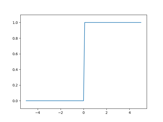
3.2.2 step関数の実装

step関数は0より上なら１それ以外は０となる活性化関数です
nxで各要素に処理を行う場合はNx.mapを使用します

activation.ex

defmodule Acivation do
  def step_function(tensor) do
    Nx.map(tensor ,fn t -> if t > 0, do: 1, else: 0 end)
  end
end

Nx.tensor([1,-1,2,0]) |> Activation.step_function()
#Nx.Tensor<
  s64[4]
  [1, 0, 1, 0]
>

3.2.3 ステップ関数のグラフ

expyplotで描画していきます
ylimの引数や他の関数の実際の使い方は以下を関数名で検索すると楽に見つけれます
https://github.com/MaxStrange/expyplot/blob/master/lib/plot.ex

またNx.tensorのままでは描画できないためNx.to_falt_listでListに変換しています

iex(1)> alias Expyplot.Plot
Expyplot.Plot
iex(2)> x = Util.arange(-5.0,5.0,0.1)
#Nx.Tensor<
  f64[101]
  [-5.0, -4.9, -4.8, -4.7, -4.6, -4.5, -4.4, -4.3, -4.2, -4.1, -4.0, -3.9, -3.8, -3.7, -3.5999999999999996, -3.5, -3.4, -3.3, -3.2, -3.0999999999999996, -3.0, -2.9, -2.8, -2.6999999999999997, -2.5999999999999996, -2.5, -2.4, -2.3, -2.1999999999999997, -2.0999999999999996, -2.0, -1.9, -1.7999999999999998, -1.6999999999999997, -1.5999999999999996, -1.5, -1.4, -1.2999999999999998, -1.1999999999999997, -1.0999999999999996, -1.0, -0.8999999999999995, -0.7999999999999998, -0.7000000000000002, -0.5999999999999996, -0.5, -0.39999999999999947, -0.2999999999999998, -0.1999999999999993, -0.09999999999999964, ...]
>
iex(3)> y = Activation.step_function(x)
#Nx.Tensor<
  f64[101]
  [0.0, 0.0, 0.0, 0.0, 0.0, 0.0, 0.0, 0.0, 0.0, 0.0, 0.0, 0.0, 0.0, 0.0, 0.0, 0.0, 0.0, 0.0, 0.0, 0.0, 0.0, 0.0, 0.0, 0.0, 0.0, 0.0, 0.0, 0.0, 0.0, 0.0, 0.0, 0.0, 0.0, 0.0, 0.0, 0.0, 0.0, 0.0, 0.0, 0.0, 0.0, 0.0, 0.0, 0.0, 0.0, 0.0, 0.0, 0.0, 0.0, 0.0, ...]
>
iex(4)> Plot.plot([Nx.to_flat_list(x),Nx.to_flat_list(y)])
"[<matplotlib.lines.Line2D object at 0x1257b8700>]"
iex(5)> Plot.ylim([-0.1,1.1])
"(-0.1, 1.1)"
iex(6)> Plot.show()

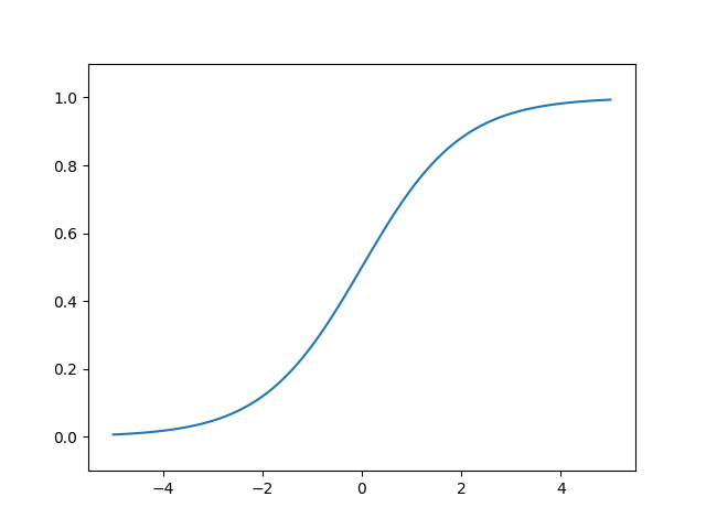
3.2.4 シグモイド関数の実装

sigmoid.py

def sigmoid(x):
  return 1 / (1 + np.exp(-x))

activation.ex

defmodule Activation do
  def sigmoid_nx(tensor) do
    Nx.divide(
      Nx.tensor(1),
      Nx.add(
        Nx.tensor(1),
        Nx.negate(tensor) |> Nx.exp()
      )
    )
  end

  def sigmoid(tensor) do
    Nx.map(tensor, fn t -> 1 / (1 + :math.exp(-t)) end)
  end
end

iex(20)> Nx.tensor([-1.0,1.0,2.0]) |> Activation.sigmoid_nx()                                                 
#Nx.Tensor<
  f64[3]
  [0.2689414213699951, 0.7310585786300049, 0.8807970779778823]
>
iex(21)> Nx.tensor([-1.0,1.0,2.0]) |> Activation.sigmoid()   
#Nx.Tensor<
  f64[3]
  [0.2689414213699951, 0.7310585786300049, 0.8807970779778823]
>

Nx.mapのほうがスッキリしていいが、sigmoid_nxのほうが早そうな気がする・・・？
好みはsigmoidほうかな

グラフ描画

iex(1)> iex(1)> alias Expyplot.Plot
Expyplot.Plot
iex(2)> x = Util.arange(-5.0,5.0,0.1)
#Nx.Tensor<
  f64[101]
  [-5.0, -4.9, -4.8, -4.7, -4.6, -4.5, -4.4, -4.3, -4.2, -4.1, -4.0, -3.9, -3.8, -3.7, -3.5999999999999996, -3.5, -3.4, -3.3, -3.2, -3.0999999999999996, -3.0, -2.9, -2.8, -2.6999999999999997, -2.5999999999999996, -2.5, -2.4, -2.3, -2.1999999999999997, -2.0999999999999996, -2.0, -1.9, -1.7999999999999998, -1.6999999999999997, -1.5999999999999996, -1.5, -1.4, -1.2999999999999998, -1.1999999999999997, -1.0999999999999996, -1.0, -0.8999999999999995, -0.7999999999999998, -0.7000000000000002, -0.5999999999999996, -0.5, -0.39999999999999947, -0.2999999999999998, -0.1999999999999993, -0.09999999999999964, ...]
>
iex(3)> y = Activation.sigmoid(x)    
#Nx.Tensor<
  f64[101]
  [0.0066928509242848554, 0.007391541344281971, 0.008162571153159897, 0.009013298652847822, 0.009951801866904324, 0.01098694263059318, 0.012128434984274237, 0.013386917827664779, 0.014774031693273055, 0.016302499371440946, 0.01798620996209156, 0.01984030573407751, 0.021881270936130476, 0.024127021417669196, 0.026596993576865863, 0.02931223075135632, 0.032295464698450516, 0.03557118927263618, 0.039165722796764356, 0.04310725494108614, 0.04742587317756678, 0.05215356307841774, 0.057324175898868755, 0.06297335605699651, 0.06913842034334684, 0.07585818002124355, 0.08317269649392238, 0.09112296101485616, 0.09975048911968518, 0.10909682119561298, 0.11920292202211755, 0.13010847436299786, 0.14185106490048782, 0.15446526508353475, 0.16798161486607557, 0.18242552380635635, 0.19781611144141825, 0.21416501695744142, 0.23147521650098238, 0.24973989440488245, 0.2689414213699951, 0.2890504973749961, 0.31002551887238755, 0.33181222783183384, 0.35434369377420466, 0.3775406687981454, 0.40131233988754816, 0.4255574831883411, 0.4501660026875223, 0.4750208125210601, ...]
>
iex(4)> Plot.plot([Nx.to_flat_list(x), Nx.to_flat_list(y)])
"[<matplotlib.lines.Line2D object at 0x13a56bdf0>]"
iex(5)> Plot.ylim([-0.1,1.1])
"(-0.1, 1.1)"
iex(6)> Plot.show()

3.2.7 ReLU関数

特に難しいことはないので関数だけ

activation.ex

defmodule Activation do
  def relu(tensor) do
    Nx.max(tensor, 0)
  end
end

3.4.3 ３層NN実装のまとめ

重みとバイアスのMapを作って|>でつなぐだけなので特に難しくはありませんね

three_layer_network.ex

defmodule ThreeLayerNetwork do
  def init_network do
    %{}
    |> Map.put(:w1, Nx.tensor([[0.1,0.3,0.5],[0.2,0.4,0.6]]))
    |> Map.put(:b1, Nx.tensor([[0.1,0.2,0.3]]))
    |> Map.put(:w2, Nx.tensor([[0.1,0.4],[0.2,0.5],[0.3,0.6]]))
    |> Map.put(:b2, Nx.tensor([[0.1,0.2]]))
    |> Map.put(:w3, Nx.tensor([[0.1,0.3],[0.2,0.4]]))
    |> Map.put(:b3, Nx.tensor([[0.1,0.2]]))
  end

  def forward(x,network) do
    [w1, w2, w3] = [network.w1, network.w2, network.w3]
    [b1, b2, b3] = [network.b1, network.b2, network.b3]

    x
    |> Nx.dot(w1)
    |> Nx.add(b1)
    |> Activation.sigmoid()
    |> Nx.dot(w2)
    |> Nx.add(b2)
    |> Activation.sigmoid()
    |> Nx.dot(w3)
    |> Nx.add(b3)
  end
end

iex(1)> network = ThreeLayerNetwork.init_network
%{b1: #Nx.Tensor<
    f64[1][3]
    [
      [0.1, 0.2, 0.3]
    ]
>, b2: #Nx.Tensor<
    f64[1][2]
    [
      [0.1, 0.2]
    ]
>, b3: #Nx.Tensor<
    f64[1][2]
    [
      [0.1, 0.2]
    ]
>, w1: #Nx.Tensor<
    f64[2][3]
    [
      [0.1, 0.3, 0.5],
      [0.2, 0.4, 0.6]
    ]
>, w2: #Nx.Tensor<
    f64[3][2]
    [
      [0.1, 0.4],
      [0.2, 0.5],
      [0.3, 0.6]
    ]
>, w3: #Nx.Tensor<
    f64[2][2]
    [
      [0.1, 0.3],
      [0.2, 0.4]
    ]
>}
iex(2)> Nx.tensor([1.0,0.5]) |> ThreeLayerNetwork.forward(network)
#Nx.Tensor<
  f64[1][2]
  [
    [0.3168270764110298, 0.6962790898619668]
  ]
>

3.5.1 恒等関数とソフトマックス関数

Nxのサンプルだと1010といった大きな数が :math.exp(1010.0)でエラーになるので
オーバーフロー対策で行列内の最大値で引いた値でsoftmaxの行列を計算します

activation.ex

defmodule Activation do
  def softmax(tensor) do
    tensor = Nx.add(tensor, Nx.reduce_max(tensor) |> Nx.negate())
    tensor
    |> Nx.exp()
    |> Nx.divide( tensor |> Nx.exp() |> Nx.sum())
  end
end

iex(1)> t = Nx.tensor([1010,1000,990]) 
#Nx.Tensor<
  s64[3]
  [1010, 1000, 990]
>
iex(2)> Nx.divide(Nx.exp( t ), Nx.sum(Nx.exp(t)))                 
** (ArithmeticError) bad argument in arithmetic expression
    (stdlib 3.14) :math.exp(1010)
    (nx 0.1.0-dev) anonymous fn/1 in Nx.BinaryBackend.exp/2
    (nx 0.1.0-dev) lib/nx/binary_backend.ex:683: Nx.BinaryBackend."-element_wise_unary_op/3-lbc$^1/2-9-"/5
    (nx 0.1.0-dev) lib/nx/binary_backend.ex:682: Nx.BinaryBackend.element_wise_unary_op/3
iex(3)> Activation.softmax(t)
#Nx.Tensor<
  f64[3]
  [0.999954600070331, 4.539786860886666e-5, 2.061060046209062e-9]
>

3.6.1 MNIST データセット 画像表示

load_mnistと画像表示は準備編で書いたので省略
https://qiita.com/the_haigo/items/1a2f0b371a3644960251#dataset-load--pil

3.6.2 ニューラルネットワークの推論処理

pklファイルの読み込みはこちらでやったので省略
https://qiita.com/the_haigo/items/1a2f0b371a3644960251#pkl%E3%83%95%E3%82%A1%E3%82%A4%E3%83%AB%E3%81%AE%E8%AA%AD%E3%81%BF%E8%BE%BC%E3%81%BF

pklファイルはこちらから
https://github.com/oreilly-japan/deep-learning-from-scratch/tree/master/ch03

test_imageのデータが0-255なので正規化する必要あるのですが、Nxに関数がないので
以下で算出しています
(& Nx.divide(&1, Nx.reduce_max(&1))).()

また全体の処理が５分くらいかかるので気長に待ってください

neuralnet_mnist.ex

defmodule NeruralnetMnist do
  def get_data() do
    x_test = Dataset.test_image() |> Nx.tensor() |> (& Nx.divide(&1, Nx.reduce_max(&1))).()
    t_test = Dataset.test_label() |> Nx.tensor()
    {x_test, t_test}
  end

  def init_network() do
    {w1,w2,w3,b1,b2,b3} = PklLoad.load("pkl/sample_weight.pkl")
    %{
      w1: Nx.tensor(w1),
      w2: Nx.tensor(w2),
      w3: Nx.tensor(w3),
      b1: Nx.tensor(b1),
      b2: Nx.tensor(b2),
      b3: Nx.tensor(b3)
    }
  end

  def predict(x, wb) do
    x
    |> Nx.dot(wb.w1)
    |> Nx.add(wb.b1)
    |> Activation.sigmoid_nx()
    |> Nx.dot(wb.w2)
    |> Nx.add(wb.b2)
    |> Activation.sigmoid_nx()
    |> Nx.dot(wb.w3)
    |> Nx.add(wb.b3)
    |> Activation.softmax()
  end

  def acc do
    {x, t} = get_data()
    IO.puts("Load Data")
    network = init_network()
    IO.puts("Load Weight")
    acc_enum(x, t, network)
   end

   def acc_enum(x,t,network) do
     {row, _} = Nx.shape(x)
     Enum.to_list(0..(row-1))
     |> Nx.tensor()
     |> Nx.map(fn i ->
       predict(x[i],network)
       |> Nx.argmax()
       |> Nx.equal(t[i])
     end)
     |> Nx.sum
     |> Nx.divide(row)
   end
end

iex(1)> NeruralnetMnist.acc
Load Data
Load Weight
#Nx.Tensor<
  f64
  0.9352
>

3.6.3 バッチ処理

Nx.to_bacthec_list(100)で
{10000,728}を {100,728} x 100のリストに変換しています
Tensorではなく、Listなので注意が必要です
Tensorだとx[0]でアクセスできたのですが、
ListなのでEnum.at(x,0)で取得する必要がありますので to_numberで変換します

Nx.argmax()ですが、本来は軸に[:y, :x]名前をつけて、axis: :xと取得するのですが、
軸名をつけてなくても indexで取得できます

defmodule NeruralnetMnist do
...
  def acc do
    {x, t} = get_data()
    IO.puts("Load Data")
    network = init_network()
    IO.puts("Load Weight")
    acc_enum_batch(x,t,network)
  end

  def acc_enum_batch(x,t,network) do
    x_b = x |> Nx.to_batched_list(100)
    t_b = t |> Nx.to_batched_list(100)
    {row, _} = x |> Nx.shape()
    batch = Enum.count(x_b)
    Enum.to_list(0..(batch-1))
    |> Nx.tensor()
    |> Nx.map(fn i ->
      predict(Enum.at(x_b,Nx.to_number(i)),network)
      |> Nx.argmax(axis: 1)
      |> Nx.equal(Enum.at(t_b,Nx.to_number(i)))
      |> Nx.sum()
    end)
    |> Nx.sum()
    |> Nx.divide(row)
  end
...
end

iex(1)> NeruralnetMnist.acc
Load Data
Load Weight
#Nx.Tensor<
  f64
  0.9352
>

補足

Elixir及びNxの製作者のJoséさんの動画では勾配の更新ですが、python的な書き方ではなく以下のようにforで回してますね
(53:00辺り)
https://www.youtube.com/watch?v=fPKMmJpAGWc

zip = Enum.zip(images, labels) |> Enum.with_index()
params =
  for e <- 1..5,
      {{images, labels}, b} <- zip,
      reduce: MNIST.init_params() do # 初期パラメーター
    params ->
      IO.puts "epoch #{e}, batch #{b}"
      MNIST.update(params, images, labels) # 勾配を求める
  end

最後に

これで３章は終了になります　お疲れさまでした
次回はbackendにgoogle xlaを使うexlaで高速化か４章をできればなーと思います

おまけ

同様のことをMatrexでやっていたのでその際のベンチになります
Matrexはcblasのnifなのでそのままで十分速いのですが、
Nxはpure elixirなのでだいぶ時間がかかっているようですね
exlaでどれだけ高速化されるか楽しみです

# Nx
Name              ips        average  deviation         median         99th %
enum          0.00480       3.47 min     ±0.00%       3.47 min       3.47 min

#Matrex
Name       ips    average deviation    median    99th %
pelemay     5.69   175.80 ms  ±7.46%   175.13 ms   227.42 ms
flow      4.89   204.30 ms  ±7.55%   203.57 ms   242.21 ms
enum      2.39   418.49 ms  ±4.62%   422.00 ms   441.99 ms 

追記

以下ご指摘を頂いてsigmoidとsoftmaxを修正しました
import Nx.defnをすればdefnで囲んだ関数は - や 1が使えるようなります

defn で定義してあげると、その中の演算子などは Nx.Defn.Kernel で定義されたものに置き換えられて、
Nx.Tensor を引数にとって計算できるようになるようです（ defn内はElixirのサブセットになる）。

activation.ex

defmodule Activation do
  import Nx.Defn
  defn sigmoid_n(tensor) do
    1 / (1 + Nx.exp(-tensor))
  end

  defn softmax_n(tensor) do
    tensor = Nx.add(tensor, -Nx.reduce_max(tensor))
    tensor
    |> Nx.exp()
    |> Nx.divide( tensor |> Nx.exp() |> Nx.sum())
  end
end

iex(1)>  Nx.tensor([-1.0,1.0,2.0]) |> Activation.sigmoid_n()
#Nx.Tensor<
  f64[3]
  [0.2689414213699951, 0.7310585786300049, 0.8807970779778823]
>
iex(2)> Nx.tensor([1010,1000,990]) |> Activation.softmax_n()
#Nx.Tensor<
  f64[3]
  [0.999954600070331, 4.539786860886666e-5, 2.061060046209062e-9]
>

コード

defnで書き直したコード
https://github.com/thehaigo/nx_dl