はじめに
webのリンク構造は手軽に遊べる大規模なネットワーク。
ネットワーク分析はwebのリンク構造で①で取得したネットワークに対して実際に分析を行なっていきます。
これも余裕で3時間以上かかる場合があるので心して試されたい。
ソースコードなどなどは筆者GitHubにご用意しております。
プログラムの概要
- 隣接行列から
networkxで有向グラフを作成 - Page rank・中心性・強連結成分分解で遊ぶ
- たのしい!!!
NetworkX
ネットワーク分析のモジュール。
- グラフのノード・エッジに複数の情報を持たせることができる。
- 中心性・強連結成分分解などのネットワーク分析を手軽に実行できる。
- 可視化が美しい。
参考サイト
レシピをまとめる余裕が無かったので、参考にさせていただいたwebサイトをまとめます。
NetworkX 公式ドキュメント
Qiita: 【Python】NetworkX 2.0の基礎的な使い方まとめ
PyQ: グラフ理論とNetworkX
DATUM STUDIO: networkxで全国名字ネットワークを可視化してみた
準備
from urllib.request import urlopen
from bs4 import BeautifulSoup

import networkx as nx

from tqdm import tqdm_notebook as tqdm
import numpy as np
from scipy import stats
import pandas as pd
pd.options.display.max_colwidth = 500

import seaborn as sns
import matplotlib.pyplot as plt
%matplotlib inline

import re
ネットワーク分析はwebのリンク構造で①に解説を掲載しています。
グラフ作成
G = nx.DiGraph()

for i in tqdm(range(len(adj))):
    for j in range(len(adj)):
        if adj[i][j]==1:
            G.add_edge(i,j)
nx.DiGraph()
有向グラフを作成。
G.add_edge(i,j)
グラフGに辺を追加する。
もっと頭のいい追加方法があるよね。うん。
グラフの特徴量計算
degree = nx.degree_centrality(G)
print("degree completed")

closeness = nx.closeness_centrality(G)
print("closeness completed")

betweenness = nx.betweenness_centrality(G)
print("betweenness completed")

pagerank = nx.pagerank(G)
print("pagerank completed")

strong_connection = sorted(nx.strongly_connected_components(G), key=lambda x: len(x), reverse=True)
print("strongly connected components completed")
nx.degree_centrality(G)
次数中心性。
各ノードの出次数と入次数の合計。
nx.degree_centrality(G)は、次数中心性の値を$n-1$で除算した値を返す。
($n$: グラフの頂点数)
nx.closeness_centrality(G)
近接中心性。
各ノードから他の全てのノードへの平均最短経路長の逆数。
nx.betweenness_centrality(G)
媒介中心性。
他の全てのノードから到達可能なノードへの最短経路が、各ノードを通る回数を割合。
nx.strongly_connected_components(G)
強連結成分分解。
sorted(nx.strongly_connected_components(G), key=lambda x: len(x), reverse=True)
とすることで、強連結成分の頂点数の多い順でソートされた配列を返す。
pandasのDataFrame作成
df = pd.DataFrame({"ID": range(len(url_list)), "URL": url_list)

df["category"] = df["URL"].apply(lambda s: s[s.index(":")+3:s.index("/", 8)])

df.loc[df['URL'] ==start_url, 'category'] = "start_page"

df["degree_centrality"] = df["ID"].map(degree)
df["closeness_centrality"] = df["ID"].map(closeness)
df["betweenness_centrality"] = df["ID"].map(betweenness)
df["Pagerank"] = df["ID"].map(pagerank)

df = df.assign(Pagerank_rank=len(df)-stats.mstats.rankdata(df["Pagerank"])+1)
df = df.assign(degree_centrality_rank=len(df)-stats.mstats.rankdata(df["degree_centrality"])+1)
df = df.assign(closeness_centrality_rank=len(df)-stats.mstats.rankdata(df["closeness_centrality"])+1)
df = df.assign(betweenness_centrality_rank=len(df)-stats.mstats.rankdata(df["betweenness_centrality"])+1)

df.to_csv(f"./{fname}.csv")
df["category"]
ネットワークの各ページをトップページごとに分類する。
ネットワーク分析はwebのリンク構造で①で、url_listには、httpで始まるURLを格納した。
これらのURLをトップページごとに分類して、categoryとする。
可視化の際に活躍する。
df.assign(Pagerank_rank=len(df)-stats.mstats.rankdata(df["###"])+1)
各種中心性のランキングを新しい列として追加する。
stats.mstats.rankdataは同じ値の順位を、それらの平均値とする。
stats.mstats.rankdataは昇順に0位から順位をとる。それらの逆順をとり、1位からの順位をDataFrameに追加する。
グラフ可視化関数
pos = nx.spring_layout(G)
nx.spring_layout(G)
グラフをいい感じにプロットする位置を計算する。
関数の外でposを定義しないと、毎回形が違うグラフが描画されてしまう。
def draw_char_graph(G, pos, title, node_type):
plt.figure(figsize=(15, 15))
nx.draw_networkx_edges(G,
pos=pos,
edge_color="gray",
edge_cmap=plt.cm.Greys,
edge_vmin=-3e4,
width=0.3,
alpha=0.2,
arrows=False)
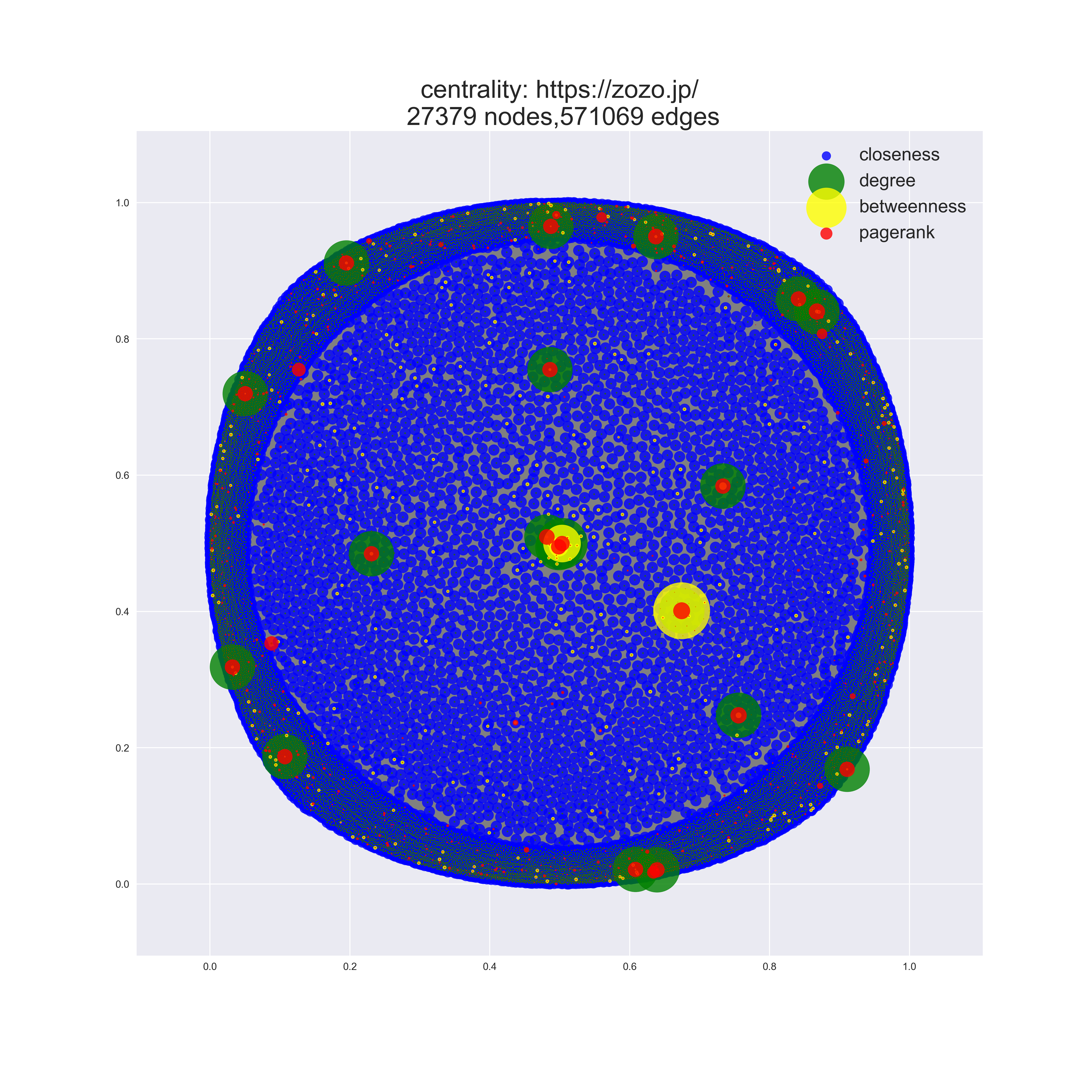
if node_type=="centrality":
node1=nx.draw_networkx_nodes(G,
pos=pos,
node_color="blue",
alpha=0.8,
node_size=[ d["closeness"]*300 for (n,d) in G.nodes(data=True)])
node2=nx.draw_networkx_nodes(G,
pos=pos,
node_color="green",
alpha=0.8,
node_size=[ d["degree"]*2000 for (n,d) in G.nodes(data=True)])
node3=nx.draw_networkx_nodes(G,
pos=pos,
node_color="yellow",
alpha=0.8,
node_size=[ d["betweenness"]*5000 for (n,d) in G.nodes(data=True)])
node4=nx.draw_networkx_nodes(G,
pos=pos,
node_color="red",
alpha=0.8,
node_size=[ d["pagerank"]*10000 for (n,d) in G.nodes(data=True)])
plt.legend([node1, node2, node3,node4], ["closeness", "degree","betweenness","pagerank"],markerscale=1,fontsize=18)
plt.title(f"centrality: {start_url}\n {nx.number_of_nodes(G)} nodes,{nx.number_of_edges(G)} edges",fontsize=25)
elif node_type=="simple":
nx.draw_networkx_nodes(G,
pos=pos,
node_color="blue",
node_size=5)
plt.title(f"{start_url}\n {nx.number_of_nodes(G)} nodes,{nx.number_of_edges(G)} edges",fontsize=25)
elif node_type=="strong_connection":
nx.draw_networkx_nodes(G,
pos=pos,
node_color="black",
node_size=10)
node1=nx.draw_networkx_nodes(G,
pos=pos,
node_color="blue",
nodelist=strong_connection[0],
node_size=30)
node2=nx.draw_networkx_nodes(G,
pos=pos,
node_color="yellow",
nodelist=strong_connection[1],
node_size=30)
node3=nx.draw_networkx_nodes(G,
pos=pos,
node_color="red",
nodelist=strong_connection[2],
node_size=30)
plt.title(f"strongly connected nodes: {title}\n {nx.number_of_nodes(G)} nodes,{nx.number_of_edges(G)} edges",fontsize=25)
plt.legend([node1, node2, node3], [f"elements: {len(strong_connection[0])} ({round(len(strong_connection[0])/nx.number_of_nodes(G)*100,2)}%)",
f"elements: {len(strong_connection[1])} ({round(len(strong_connection[1])/nx.number_of_nodes(G)*100,2)}%)",
f"elements: {len(strong_connection[2])} ({round(len(strong_connection[2])/nx.number_of_nodes(G)*100,2)}%)"],markerscale=1,fontsize=18)
plt.axis('off')
plt.savefig(f"{title}_graph_{node_type}", dpi=300)
plt.show()
draw_char_graph(G, pos, title, node_type)
グラフを描画する関数。
title
描画するグラフのタイトルと、保存するファイル名
node_type
| node_type | 描画されるグラフ |
|---|---|
"simple" |
通常のグラフ |
"centrality" |
各中心性を塗り分けたグラフ |
"strong_connection" |
強連結成分の頂点数上位3つ |
可視化
散布図
sns.pairplot(df.drop("ID", axis=1), hue='category')
plt.savefig(f'{fname}_pairplot.png')
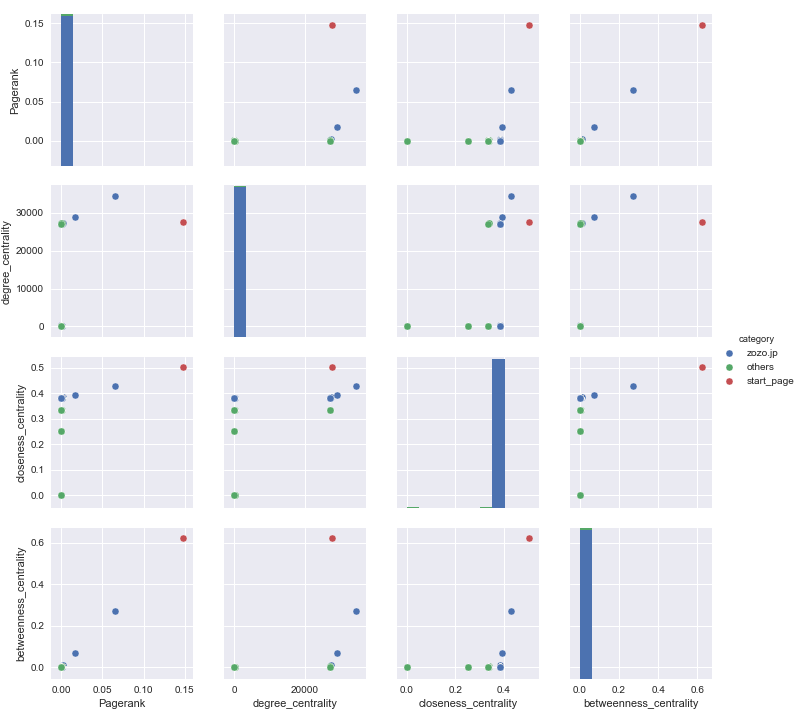
みんな大好きpairplot。
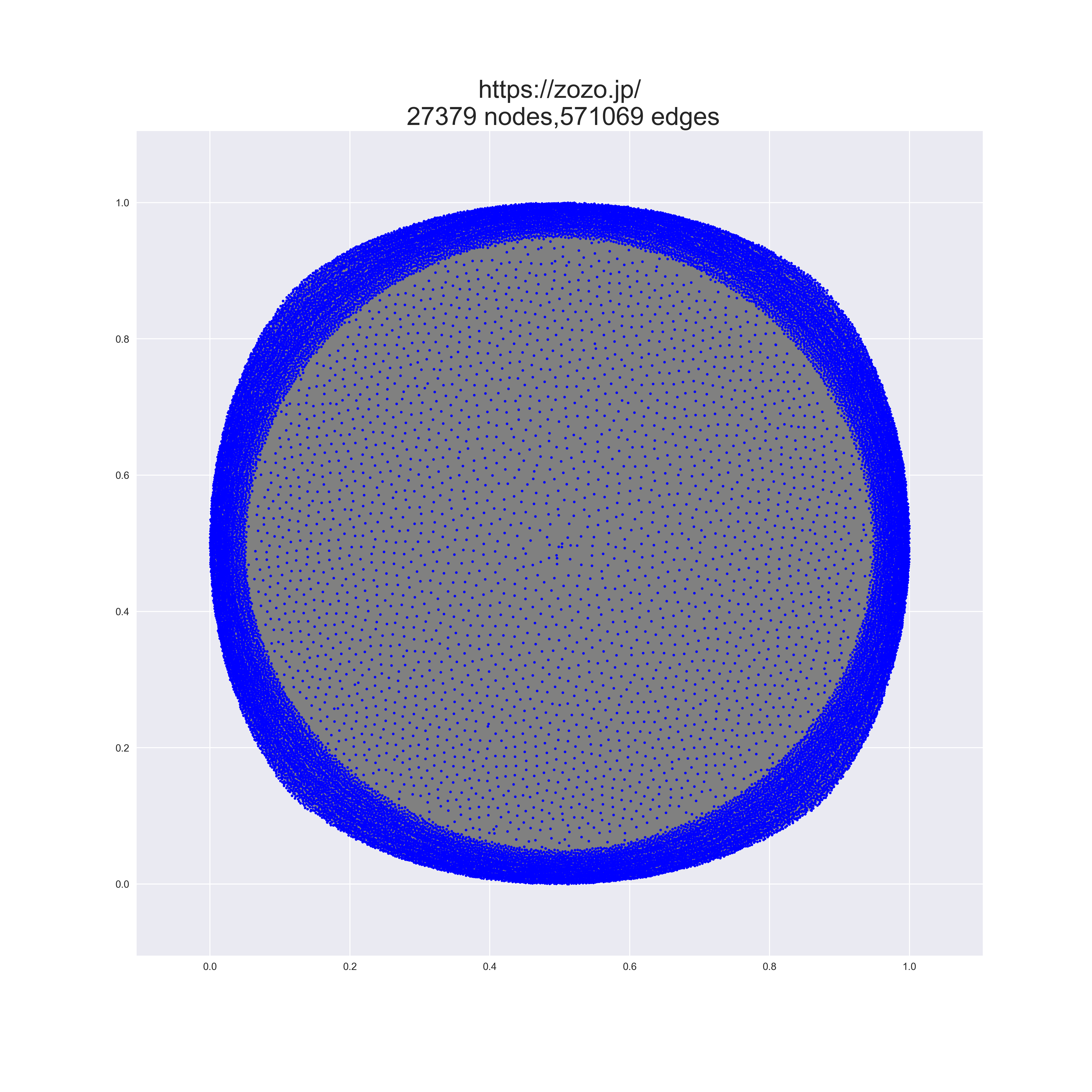
ネットワーク
draw_char_graph(G, pos, fname, node_type="simple")
draw_char_graph(G, pos, fname, node_type="centrality")
draw_char_graph(G, pos, fname, node_type="strong_connection")
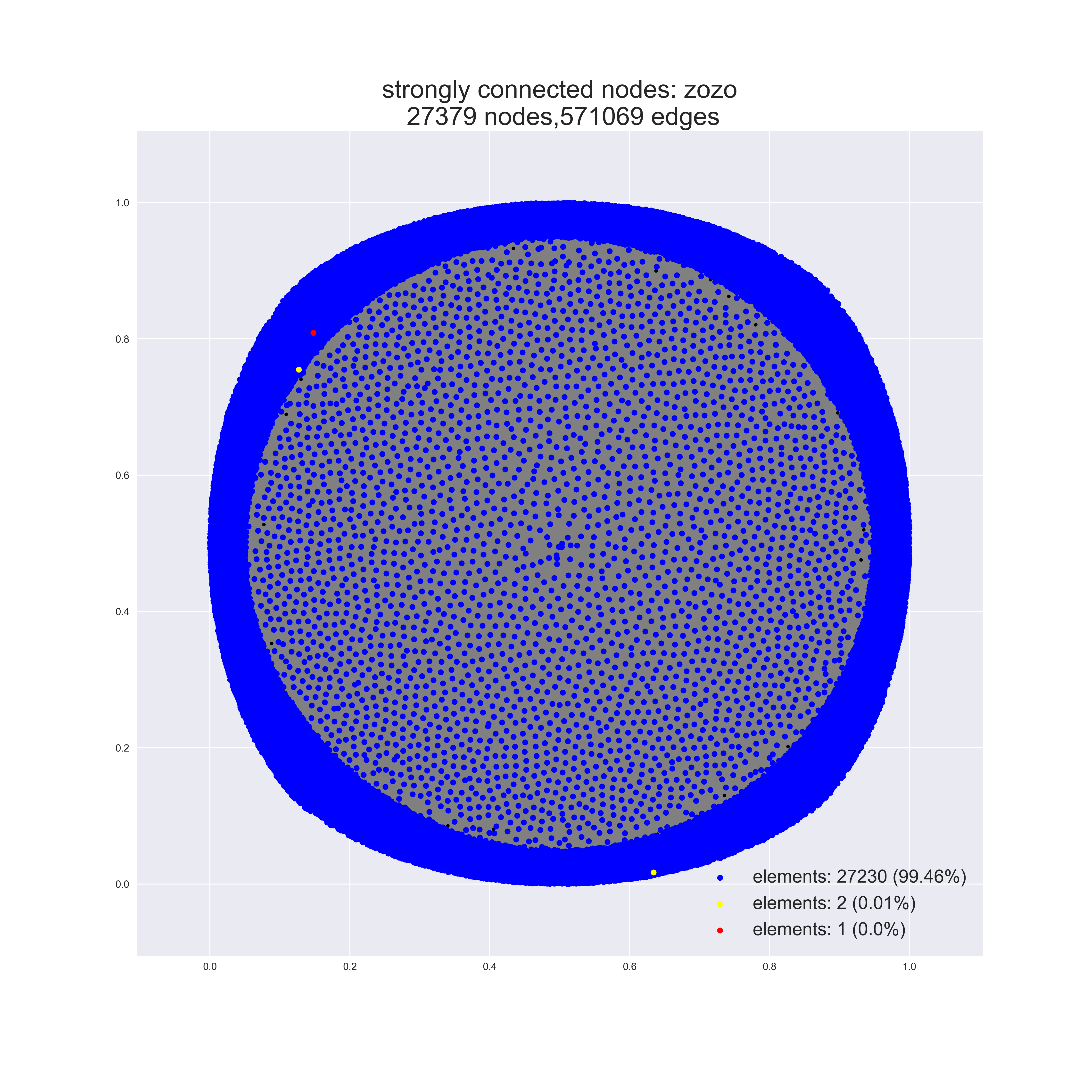
大規模すぎてよくわからん。
規模の小さなネットワークだと、ちゃんと綺麗に描画されますよ。
中心性ランキング
df_important = df[(df["Pagerank_rank"]<=10) | (df["degree_centrality_rank"]<=10) | (df["closeness_centrality_rank"]<=10) | (df["betweenness_centrality_rank"]<=10)]
df_important = df_important[["URL", "Pagerank_rank", "degree_centrality_rank", "closeness_centrality_rank", "betweenness_centrality_rank"]]

df_important.to_csv(f"./{fname}_important.csv")
たのしい!!!