DatabricksにおけるALSを用いたレコメンデーション

Posted at 2025-11-05

協調フィルタリングくらいしか知りませんでしたが、他のレコメンダーモデルを勉強する機会があったので、その結果をノートブックにまとめました。

ちなみにマニュアルにも説明がありますが、こちらのTwo TowerモデルなどはGPUが必要で、私には難解でした。

こちらのソリューションアクセラレータはまだとっつきやすいです。今回は特にALSにフォーカスしています。

データセットはこちらの化粧品レビューデータを使っています。

準備としては、上のデータをダウンロードしてデータ準備ノートブックを実行、途中でデータをUnity Catalogのボリュームにアップロードします。ノートブックの実行が終わるとテーブルが作成されます。

以降が本論となります。

Sephora スキンケアレコメンダーシステム - ALSデモ

このノートブックでは、Apache Spark MLlibのALS (Alternating Least Squares) アルゴリズムを使用して、
スキンケア製品のレコメンダーシステムを構築します。

データセット: Sephora Products and Skincare Reviews

約110万件のレビュー
約8,500製品（スキンケア製品）
ブランド、製品タイプ（モイスチャライザー、クレンザーなど）、価格情報
ユーザー属性（肌タイプ、肌色など）

実行時間: 約20-30分

推奨クラスタースペック

このノートブックを効率的に実行するための推奨クラスター構成:

最小構成（開発・検証用）

ランタイム: Databricks Runtime 14.3 LTS ML以降
ドライバー: 8コア、32GB RAM (例: m5.2xlarge)
ワーカー: 2ノード、各8コア、32GB RAM (例: m5.2xlarge)
総コア数: 24コア

推奨構成（本番・大規模データ用）

ランタイム: Databricks Runtime 14.3 LTS ML以降
ドライバー: 16コア、64GB RAM (例: m5.4xlarge)
ワーカー: 4-8ノード、各16コア、64GB RAM (例: m5.4xlarge)
総コア数: 80-144コア
オートスケーリング: 有効（4-8ノード）推奨

クラスター設定のポイント

Spark構成: デフォルトのまま（自動チューニングが有効）
適応型クエリ実行（AQE）: 有効（Databricks Runtime 10.4以降はデフォルト有効）
スポットインスタンス: コスト削減のため、ワーカーに使用可能

Sparkの並列度が処理速度に効く箇所

このノートブックでは、以下の処理でSparkの並列度が処理時間に大きく影響します：

1. ALSモデルのトレーニング（最重要）⚡

model = als.fit(training)

影響度: 最大
ALSは反復アルゴリズムで、ユーザー因子と製品因子を交互に更新
各イテレーションで大規模な行列演算が並列実行される
データ量（110万レビュー）が多いため、並列度が処理時間に直結
推奨: numUserBlocksとnumItemBlocksをクラスタのパーティション数に合わせて調整

2. 全ユーザーへの推薦生成

user_recs_raw = model.recommendForAllUsers(10)

影響度: 大
全ユーザー（数十万人）に対して並列で推薦を計算
各ユーザーごとに全製品とのスコア計算が必要

3. Window関数によるID変換

user_window = Window.orderBy("author_id")
user_indexer = reviews_clean.select("author_id").distinct()
    .withColumn("userId", (row_number().over(user_window) - 1).cast("int"))

影響度: 中〜大
distinct() + row_number().over(Window) は全データのシャッフルが発生
ソート処理が必要なため、パーティション数が影響

4. 集約処理（groupBy + agg）

review_stats = ratings.groupBy("productId").agg(
    count("rating").alias("num_reviews"),
    avg("rating").alias("avg_rating")
)

影響度: 中
groupBy().agg() はシャッフルを伴う並列集約
パーティション間でデータを再分散

5. 類似製品の類似度計算

similar_products = item_factors
    .withColumn("similarity", cosine_similarity_udf(col("features")))

影響度: 中
UDFによる全製品の類似度計算が並列実行

並列度を調整する方法

必要に応じて、以下のような調整が可能です：

# 現在のパーティション数を確認
print(f"Training data partitions: {training.rdd.getNumPartitions()}")

# 再パーティション化（クラスタのコア数の2-3倍が目安）
training = training.repartition(200)

# ALS並列度の設定
als = ALS(
    maxIter=10,
    regParam=0.1,
    rank=10,
    numUserBlocks=50,   # ユーザー行列のブロック数
    numItemBlocks=50,   # 製品行列のブロック数
    ...
)

協調フィルタリングとALS

ALSの仕組み

根本的なアプローチ:

メモリベースCF:  「似たユーザー/製品を見つける」→ 類似度を直接計算
ALS:            「ユーザーと製品の相性を予測する」→ 隠れた特徴を学習

具体例（スキンケア版）:

従来のCF:

ユーザーA: モイスチャライザーA★5, クレンザーB★5, セラムC★2
ユーザーB: モイスチャライザーA★5, クレンザーB★4, セラムC★2
→ 「AとBは似ている」→ BがアイクリームDに★5 → Aにも推薦

ALS:

レビューデータから学習:
  製品の特徴を発見 → モイスチャライザーA = [保湿力: 高, アンチエイジング: 中, 敏感肌向け: 低, ...]
  ユーザーの嗜好   → ユーザーA = [保湿好き: 高, アンチエイジング好き: 中, 敏感肌: 低, ...]

推薦時:
  アイクリームD = [保湿力: 高, アンチエイジング: 中, ...]
  ユーザーAの嗜好との相性 = 内積計算 → 高スコア → 推薦！

この「隠れた特徴」を「潜在因子」と呼びます

ALSのメリット

✅ スケーラブル: 数百万ユーザー・製品に対応可能
✅ 高精度: 潜在因子による汎化性能
✅ スパース性に強い: 評価データが少なくても機能
✅ 並列化可能: Sparkで分散処理

Sparkを使うメリット

大規模データ処理: 110万レビューを効率的に処理
統合パイプライン: データ読み込みから推薦生成まで一貫
本番移行が容易: 開発コードをそのまま本番へ
コスト効率: オートスケーリングとスポットインスタンス

内容

データセットの準備（Unity Catalogテーブル）
データの探索的分析（SQL・Python）
データの分割（トレーニング/テスト）
ALSモデルのトレーニング
モデルの評価
レコメンデーションの生成
MLflow統合
Unity Catalogモデル登録
まとめ

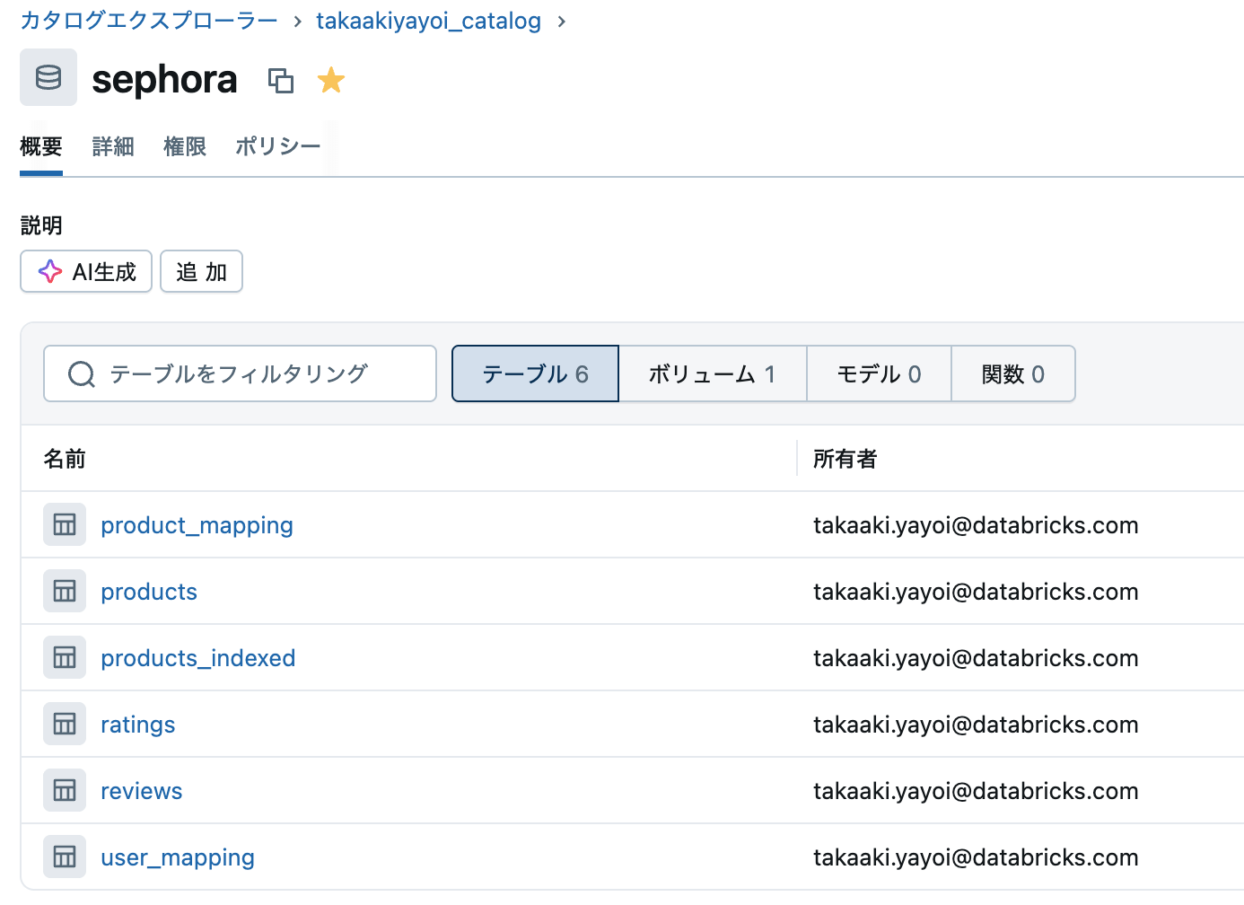
1. データセットの準備

Unity Catalogテーブルから事前に準備されたデータを読み込みます。

前提条件: sephora_data_preparation.py ノートブックを先に実行してください。

from pyspark.sql import SparkSession
from pyspark.sql.types import StructType, StructField, IntegerType, StringType, DoubleType, LongType
from pyspark.sql.functions import col, count, avg, desc, row_number
from pyspark.sql.window import Window

# Unity Catalogの設定
CATALOG_NAME = "takaakiyayoi_catalog"
SCHEMA_NAME = "sephora"

print("Unity CatalogからSephoraデータセットを読み込み中...")

# Unity Catalogテーブルからデータを読み込み
products_indexed = spark.table(f"{CATALOG_NAME}.{SCHEMA_NAME}.products_indexed")
ratings = spark.table(f"{CATALOG_NAME}.{SCHEMA_NAME}.ratings")
reviews = spark.table(f"{CATALOG_NAME}.{SCHEMA_NAME}.reviews")
user_mapping = spark.table(f"{CATALOG_NAME}.{SCHEMA_NAME}.user_mapping")
product_mapping = spark.table(f"{CATALOG_NAME}.{SCHEMA_NAME}.product_mapping")

print("データ読み込み完了!")
print(f"製品データ件数: {products_indexed.count():,}")
print(f"評価データ件数: {ratings.count():,}")
print(f"レビューデータ件数: {reviews.count():,}")
print(f"ユニークユーザー数: {user_mapping.count():,}")
print(f"ユニーク製品数: {product_mapping.count():,}")

Unity CatalogからSephoraデータセットを読み込み中...
データ読み込み完了!
製品データ件数: 2,351
評価データ件数: 1,094,411
レビューデータ件数: 1,094,411
ユニークユーザー数: 503,216
ユニーク製品数: 2,351

# データの確認
print("=== 評価データサンプル ===")
display(ratings.limit(10))

userId	productId	rating
206037	759	4
476114	759	5
339578	2016	4
110146	2016	5
407579	1265	3
227950	1265	4
205688	1265	5
115344	1265	2
363426	1876	5
277621	2184	5

print("=== 製品データサンプル ===")
display(products_indexed.limit(10))

productId	product_id_original	product_name	brand_name	price_usd	product_avg_rating	primary_category	secondary_category
0	P107306	Renewing Eye Cream	Murad	89	4.0316	Skincare	Eye Care
1	P114902	Goodbye Acne Max Complexion Correction Pads	Peter Thomas Roth	48	4.4199	Skincare	Treatments
2	P12045	Grape Water Moisturizing Face Mist	Caudalie	12	4.4431	Skincare	Moisturizers
3	P122651	Clarifying Lotion 1	CLINIQUE	20	4.515	Skincare	Cleansers
4	P122661	7 Day Face Scrub Cream Rinse-Off Formula	CLINIQUE	26	4.5321	Skincare	Cleansers
5	P122718	Exfoliating Face Scrub	CLINIQUE	26	4.6122	Skincare	Cleansers
6	P122727	Repairwear Anti-Gravity Eye Cream	CLINIQUE	54	4.1702	Skincare	Eye Care
7	P122762	Rinse-Off Foaming Cleanser	CLINIQUE	23.5	4.4933	Skincare	Cleansers
8	P122767	All About Lips	CLINIQUE	28	4.0178	Skincare	Lip Balms & Treatments
9	P122774	All About Eyes Eye Cream	CLINIQUE	37	4.0722	Skincare	Eye Care

print("=== レビューデータサンプル ===")
display(reviews.limit(10))

author_id	product_id	rating	is_recommended	review_text	review_title	skin_tone	eye_color	skin_type	hair_color
2190293206	P443842	2	false	Used to swear by this product but hate the smell of the reformulation. Love the price, but willing to spend more for a product that doesn’t smell gross	null	lightMedium	brown	combination	brown
9113341005	P443842	5	true	I’ve only been using this for a week and my skin is so much softer. It’s not as “harsh” on my skin as The Ordinary’s retinol- it took some getting used to but not this one. I’m not purging and my skin isn’t drying	More tolerable than The Ordinary	deep	brown	normal	black
23866342710	P443842	1	false	Why, why, why would you change the formula?!!! I have been using this for year. It was truly amazing. Constantly getting compliments on my skin. I am 40 years old and it was perfect. I opened my new bottle and thought I got a bad one. It was rancid. Ordered a second bottle and the same. I am so upset. Why would they change it.	New formula is awful very sad	fairLight	blue	combination	blonde
1328806527	P443842	1	false	I have used this product for years and it has been nothing short of awesome. Honestly, I am 44 and people think I am in my early 30s because of what this does for my skin. Hardly a wrinkle in sight. However, the latest package I bought in Feb 2023 contained serum that smelled rancid. Like spoiled milk. I tried it anyway and it felt thick and awful on my skin. I returned it to Sephora and learned that Inkey List REFORMULATED this product. I am SO upset. I really hope Inkey goes back to the old formulation because the new one is garbage.	Recently reformulated and the new formula is AWFUL	light	brown	combination	gray
31262847082	P443842	5	true	Great product for anti-aging Also great for dark spots	Must have product in my nighttime skincare routine	lightMedium	hazel	combination	brown
38092205147	P443842	4	true	I’ve been using this product twice a week and I’ve seen results. My skin is smothered, my pores look better and it feels healthy. You get what you pay for!	null	null	null	null	null
5090375964	P443842	4	true	Decent serum ; it didn’t cause any breakouts while using at nighttime.Just a bit heavy on my complexion.	Great size	null	brown	combination	black
42425576020	P443842	5	true	I recently bought this about less than 4 days ago, I’m not sure if there was a bad batch or what but mine does not smell of whatever everyone else is talking about. There is no smell to mine?	No smell for me!	fairLight	gray	combination	blonde
6768361454	P443842	1	false	Been using this product for well over a year and loved it. Recently restocked and thought I bought the wrong thing because it smells HORRIBLE, I can’t push through it. Idk why they would change the formula but sad I have to find a new one	null	light	hazel	combination	brown
6860968769	P443842	1	false	I used to swear by this product, but after the last purchase I made I will not be restocking this ever again. I literally thought I received something rotting inside as soon as I opened it. Shocked, I returned to the store get a new one only to open it in-store and discover the new formulation just smells like this. I literally threw up in my mouth. Save yourselves. new	Threw up in my mouth - new formulation SUCKS	lightMedium	blue	dry	brown

2. データの探索的分析

2.1 SQLを使用した基本統計

%sql
-- 基本統計情報
SELECT
  '評価データ' as metric_name,
  COUNT(*) as total_ratings,
  COUNT(DISTINCT userId) as unique_users,
  COUNT(DISTINCT productId) as unique_products,
  ROUND(AVG(rating), 2) as avg_rating,
  MIN(rating) as min_rating,
  MAX(rating) as max_rating
FROM takaakiyayoi_catalog.sephora.ratings

metric_name	total_ratings	unique_users	unique_products	avg_rating	min_rating	max_rating
評価データ	1094411	503216	2351	4.3	1	5

%sql
-- 評価値の分布
SELECT
  rating,
  COUNT(*) as count,
  ROUND(COUNT(*) * 100.0 / SUM(COUNT(*)) OVER (), 2) as percentage
FROM takaakiyayoi_catalog.sephora.ratings
GROUP BY rating
ORDER BY rating DESC

rating	count	percentage
5	698951	63.87
4	199389	18.22
3	81816	7.48
2	53032	4.85
1	61223	5.59

2.2 最もレビューされた製品

%sql
-- 最もレビューされた製品トップ10
SELECT
  p.product_name,
  p.brand_name,
  COUNT(*) as num_reviews,
  ROUND(AVG(r.rating), 2) as avg_rating,
  p.price_usd,
  p.primary_category
FROM takaakiyayoi_catalog.sephora.ratings r
JOIN takaakiyayoi_catalog.sephora.products_indexed p
  ON r.productId = p.productId
GROUP BY p.productId, p.product_name, p.brand_name, p.price_usd, p.primary_category
ORDER BY num_reviews DESC
LIMIT 10

product_name	brand_name	num_reviews	avg_rating	price_usd	primary_category
Lip Sleeping Mask Intense Hydration with Vitamin C	LANEIGE	16138	4.35	24	Skincare
Soy Hydrating Gentle Face Cleanser	fresh	8736	4.36	39	Skincare
100 percent Pure Argan Oil	Josie Maran	7763	4.5	49	Skincare
Ultra Repair Cream Intense Hydration	First Aid Beauty	7547	4.52	38	Skincare
Alpha Beta Extra Strength Daily Peel Pads	Dr. Dennis Gross Skincare	7414	4.55	92	Skincare
The True Cream Aqua Bomb	belif	7294	4.48	38	Skincare
Green Clean Makeup Removing Cleansing Balm	Farmacy	6169	4.5	36	Skincare
Green Clean Makeup Meltaway Cleansing Balm Limited Edition Jumbo	Farmacy	6169	4.5	60	Skincare
Protini Polypeptide Firming Refillable Moisturizer	Drunk Elephant	6063	3.96	68	Skincare
Superfood Antioxidant Cleanser	Youth To The People	5864	4.21	39	Skincare

2.3 カテゴリ別分析（製品タイプ別）

このデータセットはスキンケア製品に特化しており、secondary_categoryに詳細な製品タイプ（モイスチャライザー、クレンザー、セラムなど）が含まれています。

%sql
-- 製品タイプ別の統計（secondary_category）
SELECT
  p.secondary_category as product_type,
  COUNT(DISTINCT p.productId) as product_count,
  COUNT(r.rating) as total_reviews,
  ROUND(AVG(r.rating), 2) as avg_rating,
  ROUND(AVG(p.price_usd), 2) as avg_price
FROM takaakiyayoi_catalog.sephora.products_indexed p
LEFT JOIN takaakiyayoi_catalog.sephora.ratings r
  ON p.productId = r.productId
WHERE p.secondary_category IS NOT NULL
  AND p.secondary_category != ''
GROUP BY p.secondary_category
ORDER BY product_count DESC
LIMIT 15

product_type	product_count	total_reviews	avg_rating	avg_price
Moisturizers	538	297399	4.32	61.74
Treatments	452	222042	4.3	60.65
Cleansers	354	200604	4.34	36.24
Eye Care	184	74999	4.18	55.42
Value & Gift Sets	170	12099	4.27	68.72
Masks	165	70531	4.34	44.31
Mini Size	110	85498	4.29	23.32
Sunscreen	108	41139	4.17	39.31
Wellness	79	10530	4.17	40.21
High Tech Tools	76	5925	4.18	130.14
Lip Balms & Treatments	61	61688	4.33	19.26
Self Tanners	53	11942	4.08	35.83
Shop by Concern	1	15	4.27	28

2.4 ブランド別分析

%sql
-- 人気ブランドトップ15（レビュー数順）
SELECT
  p.brand_name,
  COUNT(DISTINCT p.productId) as product_count,
  COUNT(r.rating) as total_reviews,
  ROUND(AVG(r.rating), 2) as avg_rating,
  ROUND(AVG(p.price_usd), 2) as avg_price
FROM takaakiyayoi_catalog.sephora.products_indexed p
JOIN takaakiyayoi_catalog.sephora.ratings r
  ON p.productId = r.productId
WHERE p.brand_name IS NOT NULL
GROUP BY p.brand_name
ORDER BY total_reviews DESC
LIMIT 15

brand_name	product_count	total_reviews	avg_rating	avg_price
CLINIQUE	88	49029	4.25	36.39
Tatcha	40	46770	4.24	53.16
Drunk Elephant	38	42395	4.09	54.97
fresh	48	40886	4.38	46.96
The Ordinary	45	35934	4.21	11.05
Glow Recipe	27	31490	4.32	33.56
Youth To The People	27	29154	4.28	36.3
Origins	38	29063	4.36	32.44
Peter Thomas Roth	56	28846	4.32	51.96
LANEIGE	26	27519	4.37	25.88
Farmacy	23	26536	4.44	44.39
The INKEY List	41	25706	4	11.47
Sunday Riley	25	25388	4.22	80.83
OLEHENRIKSEN	31	25072	4.37	45.55
Dermalogica	48	24415	4.61	52.47

2.5 価格帯別分析

%sql
-- 価格帯別の製品数とレビュー統計
SELECT
  CASE
    WHEN price_usd < 20 THEN '0-19ドル'
    WHEN price_usd < 40 THEN '20-39ドル'
    WHEN price_usd < 60 THEN '40-59ドル'
    WHEN price_usd < 80 THEN '60-79ドル'
    WHEN price_usd < 100 THEN '80-99ドル'
    ELSE '100ドル以上'
  END as price_range,
  COUNT(DISTINCT p.productId) as product_count,
  COUNT(r.rating) as total_reviews,
  ROUND(AVG(r.rating), 2) as avg_rating
FROM takaakiyayoi_catalog.sephora.products_indexed p
LEFT JOIN takaakiyayoi_catalog.sephora.ratings r
  ON p.productId = r.productId
WHERE p.price_usd IS NOT NULL
GROUP BY
  CASE
    WHEN price_usd < 20 THEN '0-19ドル'
    WHEN price_usd < 40 THEN '20-39ドル'
    WHEN price_usd < 60 THEN '40-59ドル'
    WHEN price_usd < 80 THEN '60-79ドル'
    WHEN price_usd < 100 THEN '80-99ドル'
    ELSE '100ドル以上'
  END
ORDER BY
  CASE price_range
    WHEN '0-19ドル' THEN 1
    WHEN '20-39ドル' THEN 2
    WHEN '40-59ドル' THEN 3
    WHEN '60-79ドル' THEN 4
    WHEN '80-99ドル' THEN 5
    ELSE 6
  END

price_range	product_count	total_reviews	avg_rating
0-19ドル	341	184417	4.26
20-39ドル	731	372559	4.28
40-59ドル	494	231895	4.32
60-79ドル	359	161393	4.33
80-99ドル	177	79193	4.35
100ドル以上	249	64954	4.27

2.6 高評価製品の分析

%sql
-- 高評価製品トップ10（レビュー数10件以上）
SELECT
  p.product_name,
  p.brand_name,
  COUNT(*) as num_reviews,
  ROUND(AVG(r.rating), 2) as avg_rating,
  p.price_usd,
  p.primary_category
FROM takaakiyayoi_catalog.sephora.ratings r
JOIN takaakiyayoi_catalog.sephora.products_indexed p
  ON r.productId = p.productId
GROUP BY p.productId, p.product_name, p.brand_name, p.price_usd, p.primary_category
HAVING COUNT(*) >= 10
ORDER BY avg_rating DESC, num_reviews DESC
LIMIT 10

product_name	brand_name	num_reviews	avg_rating	price_usd	primary_category
Skin Filter Daily Brightening Phyto-Retinol + AHA Serum	The Nue Co.	17	5	65	Skincare
LUNA 4 Facial Cleansing & Firming Massage for Balanced Skin	FOREO	16	5	279	Skincare
Liquid Gold Midnight Reboot Serum with 14% Glycolic Acid and Tripeptide-5	Alpha-H	16	5	105	Skincare
Barrier Culture Moisturizer with Niacinamide & Squalane	The Nue Co.	12	5	65	Skincare
Barrier Culture Cleanser Pre-, Pro- & Postbiotic Face Wash	The Nue Co.	11	5	42	Skincare
Youth Reformer Firming Vitamin C Oil Serum	FaceGym	53	4.96	110	Skincare
Multi Action Clear Acne Control 30-Day Trial Kit	StriVectin	24	4.96	39	Skincare
Mini Evening Primrose + Green Tea Algae Retinol Face Oil	MARA	78	4.95	66	Skincare
Evening Primrose + Green Tea Algae Retinol Face Oil	MARA	78	4.95	120	Skincare
Tan Build Up Remover Mitt	St. Tropez	59	4.95	9	Skincare

3. データの分割

トレーニングデータとテストデータに分割します（80:20）

# データをトレーニングとテストに分割
(training, test) = ratings.randomSplit([0.8, 0.2], seed=42)

print(f"トレーニングデータ: {training.count():,} 件")
print(f"テストデータ: {test.count():,} 件")

トレーニングデータ: 876,200 件
テストデータ: 218,211 件

4. ALSモデルのトレーニング

製品レコメンデーションのためにALSモデルをトレーニングします。

パラメータ:

maxIter: イテレーション数
regParam: 正則化パラメータ（過学習を防ぐ）
rank: 潜在因子の数
coldStartStrategy: 新規ユーザー/製品の扱い

from pyspark.ml.recommendation import ALS
from pyspark.ml.evaluation import RegressionEvaluator
import mlflow
import mlflow.spark

# MLflow実験の設定
mlflow.set_experiment("/Users/takaaki.yayoi@databricks.com/20251104_sephora_als/sephora_recommender_experiment")

print("ALSモデルのトレーニング開始...")

# MLflowで実験を記録
with mlflow.start_run(run_name="sephora_als_baseline") as run:

    # パラメータの設定
    max_iter = 10
    reg_param = 0.1
    rank = 10

    # データセットのリネージを記録
    training_dataset = mlflow.data.from_spark(
        training,
        table_name=f"{CATALOG_NAME}.{SCHEMA_NAME}.ratings",
        version="0"
    )
    mlflow.log_input(training_dataset, context="training")

    test_dataset = mlflow.data.from_spark(
        test,
        table_name=f"{CATALOG_NAME}.{SCHEMA_NAME}.ratings",
        version="0"
    )
    mlflow.log_input(test_dataset, context="validation")

    # ALSモデルの構築
    als = ALS(
        maxIter=max_iter,
        regParam=reg_param,
        rank=rank,
        userCol="userId",
        itemCol="productId",
        ratingCol="rating",
        coldStartStrategy="drop",
        nonnegative=True
    )

    # パラメータをMLflowにロギング
    mlflow.log_param("maxIter", max_iter)
    mlflow.log_param("regParam", reg_param)
    mlflow.log_param("rank", rank)
    mlflow.log_param("coldStartStrategy", "drop")
    mlflow.log_param("nonnegative", True)

    # データセット情報をロギング
    mlflow.log_param("training_count", training.count())
    mlflow.log_param("test_count", test.count())

    # モデルのトレーニング
    model = als.fit(training)

    print("トレーニング完了!")
    print(f"MLflow Run ID: {run.info.run_id}")

    # 評価指標の計算用evaluatorを準備
    evaluator = RegressionEvaluator(
        metricName="rmse",
        labelCol="rating",
        predictionCol="prediction"
    )

    # テストデータで予測
    predictions = model.transform(test)

    # RMSEを計算
    rmse = evaluator.evaluate(predictions)

    # メトリクスをMLflowにロギング
    mlflow.log_metric("rmse", rmse)
    mlflow.log_metric("test_rmse", rmse)

    # 追加のメトリクス（MAE）も計算してロギング
    evaluator_mae = RegressionEvaluator(
        metricName="mae",
        labelCol="rating",
        predictionCol="prediction"
    )
    mae = evaluator_mae.evaluate(predictions)
    mlflow.log_metric("mae", mae)

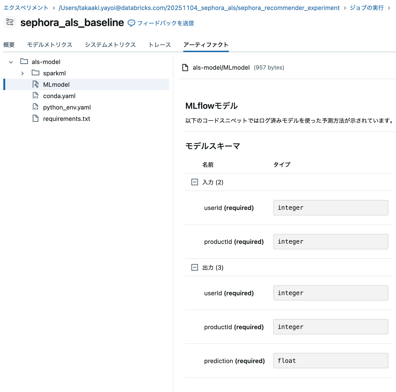
    # モデルのsignatureを作成（Unity Catalog登録用）
    from mlflow.models import infer_signature

    # サンプル入力データ（userId, productId）
    sample_input = test.select("userId", "productId").limit(10).toPandas()
    # サンプル出力データ（予測結果）
    sample_output = predictions.select("userId", "productId", "prediction").limit(10).toPandas()

    # signatureを推論
    signature = infer_signature(sample_input, sample_output)

    # モデルをMLflowに保存（signatureを含める）
    mlflow.spark.log_model(
        model,
        "als-model",
        signature=signature,
        registered_model_name=None
    )

    print(f"テストデータのRMSE = {rmse:.3f}")
    print(f"テストデータのMAE = {mae:.3f}")
    print(f"✓ モデルをsignature付きで保存しました")

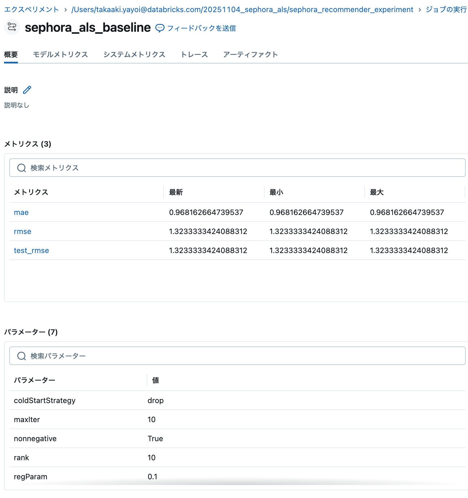
テストデータのRMSE = 1.323
テストデータのMAE = 0.968
✓ モデルをsignature付きで保存しました

MLflowのエクスペリメントからモデルに関する情報を確認できます。

5. モデルの評価

RMSE (Root Mean Squared Error) を使用してモデルの性能を評価します。

# 予測結果の確認
print("=== 予測結果サンプル ===")
display(
    predictions
    .join(products_indexed, "productId")
    .select("userId", "product_name", "brand_name", "rating", "prediction")
    .limit(10)
)

=== 予測結果サンプル ===

userId	product_name	brand_name	rating	prediction
31	Take The Day Off Cleansing Balm Makeup Remover	CLINIQUE	5	4.812748432159424
53	Niacinamide 10% + Zinc 1% Oil Control Serum	The Ordinary	5	2.2006661891937256
78	Midnight Recovery Concentrate Moisturizing Face Oil	Kiehl's Since 1851	2	2.1206536293029785
85	Lala Retro Whipped Refillable Moisturizer with Ceramides	Drunk Elephant	5	3.8595359325408936
108	Vinosource-Hydra Moisturizing Sorbet	Caudalie	5	3.5733797550201416
321	Santorini Grape Poreless Skin Cream	KORRES	5	3.796710968017578
322	Balancing Force Oil Control Toner	OLEHENRIKSEN	5	2.9253413677215576
471	Mini Superfood Antioxidant Cleanser	Youth To The People	5	4.6766791343688965
580	Even Smoother Glycolic Retinol Resurfacing Serum	Peter Thomas Roth	5	4.7179436683654785
580	Cold Plunge Pore Remedy Moisturizer with BHA/LHA	OLEHENRIKSEN	5	3.7894437313079834

5.1 モデル結果の可視化

import plotly.graph_objects as go
import plotly.express as px
from plotly.subplots import make_subplots
import numpy as np

# Pandasに変換して可視化（サンプリングして軽量化）
predictions_pd = predictions.select("rating", "prediction").sample(fraction=0.1, seed=42).limit(10000).toPandas()
errors = predictions_pd['rating'] - predictions_pd['prediction']

# サブプロット作成
fig = make_subplots(
    rows=2, cols=2,
    subplot_titles=(
        '予測 vs 実際の評価（散布図）',
        f'予測誤差の分布（平均: {errors.mean():.3f}）',
        '評価分布の比較',
        '評価値ごとの予測分布'
    ),
    specs=[[{"type": "scatter"}, {"type": "histogram"}],
           [{"type": "histogram"}, {"type": "box"}]]
)

# 1. 予測 vs 実際の評価 - 散布図
fig.add_trace(
    go.Scatter(
        x=predictions_pd['rating'],
        y=predictions_pd['prediction'],
        mode='markers',
        marker=dict(size=3, opacity=0.3, color='blue'),
        name='予測',
        showlegend=True
    ),
    row=1, col=1
)
# 理想的な予測線
fig.add_trace(
    go.Scatter(
        x=[1, 5], y=[1, 5],
        mode='lines',
        line=dict(color='red', dash='dash', width=2),
        name='理想的な予測',
        showlegend=True
    ),
    row=1, col=1
)

# 2. 予測誤差のヒストグラム
fig.add_trace(
    go.Histogram(
        x=errors,
        nbinsx=50,
        marker=dict(color='skyblue', line=dict(color='black', width=1)),
        name='誤差分布',
        showlegend=False
    ),
    row=1, col=2
)

# 3. 実際の評価の分布 vs 予測の評価の分布
fig.add_trace(
    go.Histogram(
        x=predictions_pd['rating'],
        nbinsx=5,
        marker=dict(color='green', opacity=0.5, line=dict(color='black', width=1)),
        name='実際の評価'
    ),
    row=2, col=1
)
fig.add_trace(
    go.Histogram(
        x=predictions_pd['prediction'],
        nbinsx=20,
        marker=dict(color='orange', opacity=0.5, line=dict(color='black', width=1)),
        name='予測評価'
    ),
    row=2, col=1
)

# 4. 評価値ごとの予測分布（ボックスプロット）
for rating in sorted(predictions_pd['rating'].unique()):
    fig.add_trace(
        go.Box(
            y=predictions_pd[predictions_pd['rating'] == rating]['prediction'],
            name=f'評価{int(rating)}',
            marker=dict(color='lightblue'),
            showlegend=False
        ),
        row=2, col=2
    )

# レイアウト設定
fig.update_xaxes(title_text="実際の評価", row=1, col=1)
fig.update_yaxes(title_text="予測評価", row=1, col=1)
fig.update_xaxes(title_text="誤差（実際 - 予測）", row=1, col=2)
fig.update_yaxes(title_text="頻度", row=1, col=2)
fig.update_xaxes(title_text="評価値", row=2, col=1)
fig.update_yaxes(title_text="頻度", row=2, col=1)
fig.update_xaxes(title_text="実際の評価", row=2, col=2)
fig.update_yaxes(title_text="予測評価の分布", row=2, col=2)

fig.update_layout(
    height=900,
    width=1400,
    title_text="<b>モデル評価の可視化（サンプル）</b>",
    showlegend=True,
    font=dict(size=12)
)

fig.show(config={'displayModeBar': True})

print(f"\n=== 予測精度の統計 ===")
print(f"誤差の平均: {errors.mean():.3f}")
print(f"誤差の標準偏差: {errors.std():.3f}")
print(f"平均絶対誤差 (MAE): {abs(errors).mean():.3f}")

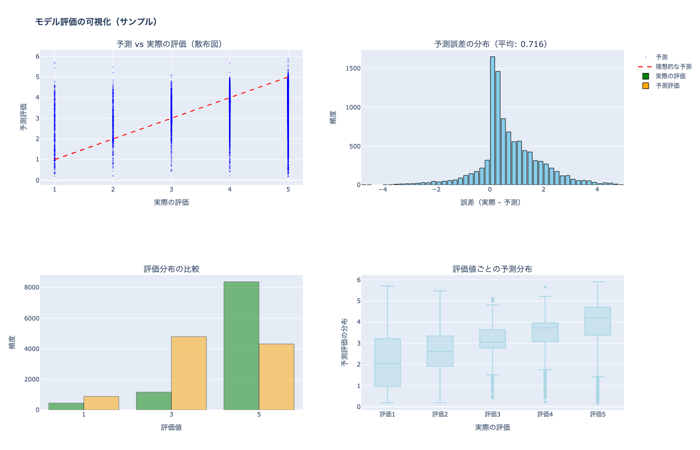
=== 予測精度の統計 ===
誤差の平均: 0.716
誤差の標準偏差: 1.136
平均絶対誤差 (MAE): 0.980

5.2 データ分析の可視化

# レビュー数の分析
product_stats = ratings.groupBy("productId").agg(
    count("rating").alias("num_reviews"),
    avg("rating").alias("avg_rating")
).toPandas()

# サブプロット作成
fig = make_subplots(
    rows=1, cols=2,
    subplot_titles=(
        '製品の人気度分布（ロングテール）',
        'レビュー数 vs 平均評価'
    )
)

# 1. 製品ごとのレビュー数分布
sorted_counts = product_stats['num_reviews'].sort_values(ascending=False).values
fig.add_trace(
    go.Scatter(
        x=list(range(len(sorted_counts))),
        y=sorted_counts,
        mode='lines',
        line=dict(color='blue', width=2),
        name='レビュー数',
        showlegend=True
    ),
    row=1, col=1
)
# 中央値の線
median_val = product_stats['num_reviews'].median()
fig.add_trace(
    go.Scatter(
        x=[0, len(sorted_counts)],
        y=[median_val, median_val],
        mode='lines',
        line=dict(color='red', dash='dash', width=2),
        name=f'中央値: {median_val:.0f}',
        showlegend=True
    ),
    row=1, col=1
)

# 2. 平均評価とレビュー数の関係
fig.add_trace(
    go.Scatter(
        x=product_stats['num_reviews'],
        y=product_stats['avg_rating'],
        mode='markers',
        marker=dict(size=5, opacity=0.5, color='purple'),
        name='製品',
        showlegend=True
    ),
    row=1, col=2
)

# レイアウト設定
fig.update_xaxes(title_text="製品のランク", row=1, col=1)
fig.update_yaxes(title_text="レビュー数", type="log", row=1, col=1)
fig.update_xaxes(title_text="レビュー数", type="log", row=1, col=2)
fig.update_yaxes(title_text="平均評価", row=1, col=2)

fig.update_layout(
    height=600,
    width=1400,
    title_text="<b>レビューデータの分析</b>",
    showlegend=True,
    font=dict(size=12)
)

fig.show(config={'displayModeBar': True})

print(f"\n=== データセットの特徴 ===")
print(f"レビュー数の中央値: {product_stats['num_reviews'].median():.0f}")
print(f"上位20%の製品が全レビューの{(product_stats.nlargest(int(len(product_stats)*0.2), 'num_reviews')['num_reviews'].sum() / product_stats['num_reviews'].sum() * 100):.1f}%を占める")

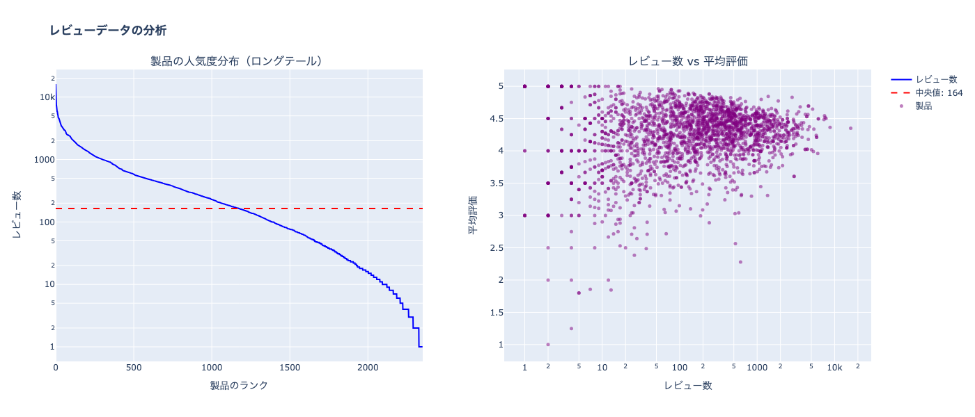
=== データセットの特徴 ===
レビュー数の中央値: 164
上位20%の製品が全レビューの72.4%を占める

6. レコメンデーションの生成

各ユーザーにトップ10の製品を推薦します。

予測評価スコアとは

予測評価スコア = 「このユーザーがこの製品を使用したら、何点の評価をつけるか」の予測値

# 全ユーザーに対してトップ10の製品を推薦
user_recs_raw = model.recommendForAllUsers(10)

# 推薦スコアを1-5の範囲にクリップする（構造体の配列を展開して処理）
from pyspark.sql.functions import explode, struct, collect_list, least, greatest, lit

user_recs = (
    user_recs_raw
    .select(col("userId"), explode(col("recommendations")).alias("rec"))
    .select(
        col("userId"),
        col("rec.productId").alias("productId"),
        # スコアを1-5にクリップ
        least(greatest(col("rec.rating"), lit(1.0)), lit(5.0)).alias("rating")
    )
    # 再度構造体に変換
    .groupBy("userId")
    .agg(collect_list(struct(col("productId"), col("rating"))).alias("recommendations"))
)

# 存在するユーザーIDをサンプル取得（トレーニングデータに存在するユーザー）
sample_user_id = training.select("userId").distinct().first()[0]
print(f"=== ユーザー{sample_user_id}への推薦製品 ===")

# 推薦結果を見やすく表示
user_recs_expanded = (
    user_recs
    .filter(col("userId") == sample_user_id)
    .select(col("userId"), explode(col("recommendations")).alias("rec"))
    .select(
        col("userId"),
        col("rec.productId").alias("productId"),
        col("rec.rating").alias("predicted_rating")
    )
    .join(products_indexed, "productId")
    .select("userId", "product_name", "brand_name", "price_usd", "predicted_rating")
)

display(user_recs_expanded)

=== ユーザー0への推薦製品 ===

product_name	brand_name	price_usd	predicted_rating
Acne Treatment Gel	SEPHORA COLLECTION	20	5
Trinity+ Starter Kit	NuFACE	395	5
Refreshing Water Sunscreen Stick SPF 50	COOLA	30	5
Glycolic Eye Cream	Mario Badescu	20	5
Crystal Facial Roller Set	SEPHORA COLLECTION	35	5
Dior Skin Mattifying Papers	Dior	35	5
The Bright Set	The Ordinary	40.7	5
DelIKate Try Me Kit	Kate Somerville	49	5
Anti-Aging Regimen Kit	Mario Badescu	30	5
Rose Hydration Pore-Minimizing Mist	fresh	24	5

6.1 推薦結果の可視化

# 複数ユーザーの推薦スコアを可視化
# トレーニングデータから実際に存在するユーザーを3人サンプル
sample_users = [row[0] for row in training.select("userId").distinct().limit(3).collect()]

# サブプロット作成（2x2レイアウト）
fig = make_subplots(
    rows=2, cols=2,
    subplot_titles=[f'ユーザー {uid} への推薦' for uid in sample_users] + ['全推薦スコアの分布'],
    specs=[[{"type": "bar"}, {"type": "bar"}],
           [{"type": "bar"}, {"type": "histogram"}]]
)

# 各ユーザーの推薦を可視化
positions = [(1,1), (1,2), (2,1)]
for idx, (user_id, pos) in enumerate(zip(sample_users, positions)):
    # ユーザーの推薦を取得
    user_rec_pd = (
        user_recs
        .filter(col("userId") == user_id)
        .select(explode(col("recommendations")).alias("rec"))
        .select(
            col("rec.productId").alias("productId"),
            col("rec.rating").alias("predicted_rating")
        )
        .join(products_indexed, "productId")
        .select("product_name", "predicted_rating")
        .toPandas()
    )

    # タイトルを短縮（より長く表示）
    user_rec_pd['short_name'] = user_rec_pd['product_name'].apply(
        lambda x: x[:40] + '...' if len(x) > 40 else x
    )

    # 横棒グラフで表示
    fig.add_trace(
        go.Bar(
            y=user_rec_pd['short_name'][::-1],
            x=user_rec_pd['predicted_rating'][::-1],
            orientation='h',
            marker=dict(color='steelblue'),
            showlegend=False,
            hovertemplate='<b>%{y}</b><br>スコア: %{x:.2f}<extra></extra>'
        ),
        row=pos[0], col=pos[1]
    )

    fig.update_xaxes(title_text="予測評価スコア", row=pos[0], col=pos[1])

# 6番目のサブプロット：全体の推薦スコア分布（サンプリングして軽量化）
all_recs_pd = (
    user_recs
    .sample(fraction=0.1, seed=42)  # 10%をサンプリング
    .select(explode(col("recommendations")).alias("rec"))
    .select(col("rec.rating").alias("predicted_rating"))
    .limit(10000)  # 最大10,000件に制限
    .toPandas()
)

fig.add_trace(
    go.Histogram(
        x=all_recs_pd['predicted_rating'],
        nbinsx=50,
        marker=dict(color='coral', line=dict(color='black', width=1)),
        showlegend=False
    ),
    row=2, col=2
)

fig.update_xaxes(title_text="予測評価スコア", row=2, col=2)
fig.update_yaxes(title_text="頻度", row=2, col=2)

# レイアウト設定（見やすく大きく）
fig.update_layout(
    height=900,
    width=1400,
    title_text="<b>ユーザーへの推薦結果（サンプル）</b>",
    showlegend=False,
    font=dict(size=12)
)

# 軽量化設定
fig.show(config={'displayModeBar': True})

print(f"\n=== 推薦スコアの統計 ===")
print(f"最小値: {all_recs_pd['predicted_rating'].min():.3f}")
print(f"最大値: {all_recs_pd['predicted_rating'].max():.3f}")
print(f"平均値: {all_recs_pd['predicted_rating'].mean():.3f}")
print(f"中央値: {all_recs_pd['predicted_rating'].median():.3f}")

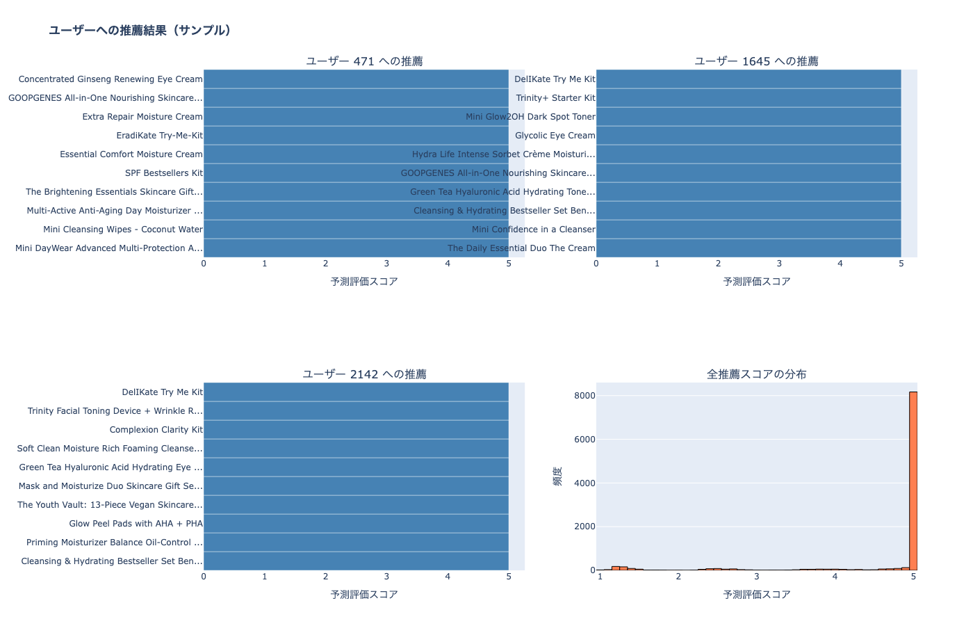
=== 推薦スコアの統計 ===
最小値: 1.000
最大値: 5.000
平均値: 4.624
中央値: 5.000

6.2 推薦の多様性とカバレッジ分析

# 推薦された製品の統計
recommended_products = (
    user_recs
    .select(explode(col("recommendations")).alias("rec"))
    .select(col("rec.productId").alias("productId"))
    .distinct()
)

total_products = products_indexed.count()
recommended_count = recommended_products.count()
coverage = (recommended_count / total_products) * 100

# 推薦頻度の分析
rec_frequency = (
    user_recs
    .select(explode(col("recommendations")).alias("rec"))
    .groupBy(col("rec.productId").alias("productId"))
    .agg(count("*").alias("recommendation_count"))
    .join(products_indexed, "productId")
    .orderBy(desc("recommendation_count"))
)

top_recommended = rec_frequency.limit(20).toPandas()

# タイトルを短縮
top_recommended['short_name'] = top_recommended['product_name'].apply(
    lambda x: x[:40] + '...' if len(x) > 40 else x
)

# サブプロット作成
fig = make_subplots(
    rows=1, cols=2,
    subplot_titles=(
        '最も推薦された製品トップ20',
        f'推薦カバレッジ: {coverage:.1f}%'
    ),
    specs=[[{"type": "bar"}, {"type": "pie"}]]
)

# 1. 最も推薦された製品トップ20
fig.add_trace(
    go.Bar(
        y=top_recommended['short_name'][::-1],
        x=top_recommended['recommendation_count'][::-1],
        orientation='h',
        marker=dict(color='teal'),
        showlegend=False,
        hovertemplate='<b>%{y}</b><br>推薦回数: %{x}<extra></extra>'
    ),
    row=1, col=1
)

fig.update_xaxes(title_text="推薦回数", row=1, col=1)

# 2. 推薦カバレッジ（円グラフ）
fig.add_trace(
    go.Pie(
        labels=[f'推薦された ({recommended_count}製品)', f'推薦されない ({total_products - recommended_count}製品)'],
        values=[recommended_count, total_products - recommended_count],
        marker=dict(colors=['#ff9999', '#66b3ff']),
        textinfo='percent+label',
        textfont=dict(size=11),
        pull=[0.1, 0],
        showlegend=True
    ),
    row=1, col=2
)

# レイアウト設定
fig.update_layout(
    height=700,
    width=1400,
    title_text="<b>推薦の多様性とカバレッジ分析</b>",
    font=dict(size=12)
)

fig.show(config={'displayModeBar': True})

print(f"\n=== 推薦の多様性 ===")
print(f"全製品数: {total_products}")
print(f"推薦された製品数: {recommended_count}")
print(f"カバレッジ: {coverage:.1f}%")

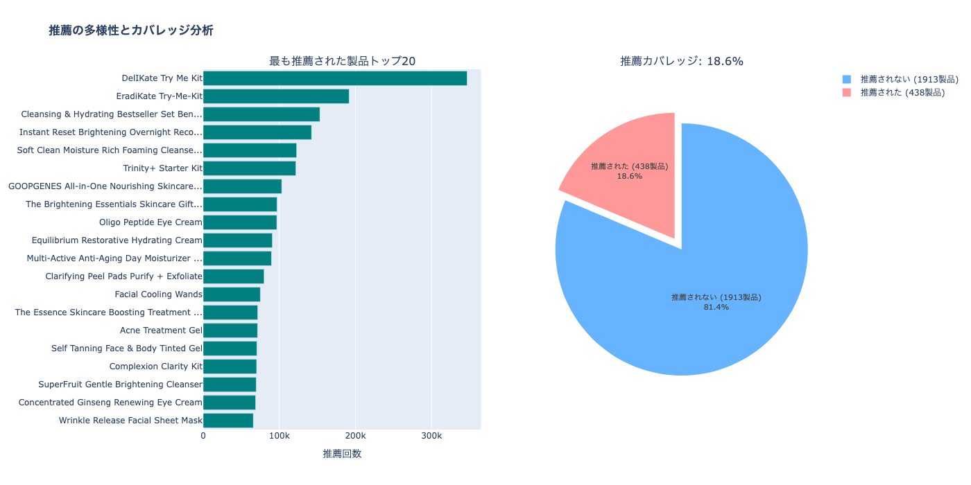
=== 推薦の多様性 ===
全製品数: 2351
推薦された製品数: 438
カバレッジ: 18.6%

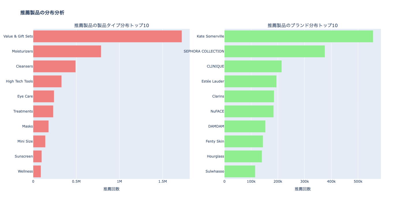
6.3 製品タイプ別・ブランド別の推薦分析

# 推薦されている製品の製品タイプ分布（secondary_category）
rec_type_dist = (
    user_recs
    .select(explode(col("recommendations")).alias("rec"))
    .select(col("rec.productId").alias("productId"))
    .join(products_indexed, "productId")
    .filter(col("secondary_category").isNotNull())
    .filter(col("secondary_category") != "")
    .groupBy("secondary_category")
    .agg(count("*").alias("recommendation_count"))
    .orderBy(desc("recommendation_count"))
    .limit(10)
    .toPandas()
)

# 製品タイプ分布を表示
print(f"\n=== 製品タイプ分布 ===")
print(rec_type_dist)

# 推薦されている製品のブランド分布
rec_brand_dist = (
    user_recs
    .select(explode(col("recommendations")).alias("rec"))
    .select(col("rec.productId").alias("productId"))
    .join(products_indexed, "productId")
    .groupBy("brand_name")
    .agg(count("*").alias("recommendation_count"))
    .orderBy(desc("recommendation_count"))
    .limit(10)
    .toPandas()
)

# サブプロット作成
fig = make_subplots(
    rows=1, cols=2,
    subplot_titles=(
        '推薦製品の製品タイプ分布トップ10',
        '推薦製品のブランド分布トップ10'
    ),
    specs=[[{"type": "bar"}, {"type": "bar"}]]
)

# 1. 製品タイプ分布
fig.add_trace(
    go.Bar(
        y=rec_type_dist['secondary_category'][::-1],
        x=rec_type_dist['recommendation_count'][::-1],
        orientation='h',
        marker=dict(color='lightcoral'),
        showlegend=False,
        hovertemplate='<b>%{y}</b><br>推薦回数: %{x}<extra></extra>'
    ),
    row=1, col=1
)

# 2. ブランド分布
fig.add_trace(
    go.Bar(
        y=rec_brand_dist['brand_name'][::-1],
        x=rec_brand_dist['recommendation_count'][::-1],
        orientation='h',
        marker=dict(color='lightgreen'),
        showlegend=False,
        hovertemplate='<b>%{y}</b><br>推薦回数: %{x}<extra></extra>'
    ),
    row=1, col=2
)

fig.update_xaxes(title_text="推薦回数", row=1, col=1)
fig.update_xaxes(title_text="推薦回数", row=1, col=2)

# レイアウト設定
fig.update_layout(
    height=700,
    width=1400,
    title_text="<b>推薦製品の分布分析</b>",
    font=dict(size=12)
)

fig.show(config={'displayModeBar': True})

=== 製品タイプ分布 ===
  secondary_category  recommendation_count
0  Value & Gift Sets               1723190
1       Moisturizers                787416
2          Cleansers                491919
3    High Tech Tools                328929
4           Eye Care                241887
5         Treatments                232799
6              Masks                178930
7          Mini Size                141027
8          Sunscreen                 98613
9           Wellness                 89103

7. MLflowでのモデル管理

モデルは既にMLflowに保存されています！

MLflowでの確認方法

左サイドバーの「Experiments」をクリック
実験名: /Users/takaaki.yayoi@databricks.com/20251104_sephora_als/sephora_recommender_experiment
各Runをクリックすると以下が確認できます：
- Parameters: maxIter, regParam, rank など
- Metrics: RMSE, MAE
- Artifacts: 保存されたモデル

8. Unity Catalogへのモデル登録

モデルをUnity Catalogに登録することで、以下のメリットがあります：

バージョン管理: モデルのバージョンを一元管理
ガバナンス: アクセス制御とリネージ追跡
本番デプロイ: Model Servingとの統合
共同作業: チーム間でのモデル共有

import mlflow
from mlflow.tracking import MlflowClient

# Unity Catalogのモデル名
UC_MODEL_NAME = f"{CATALOG_NAME}.{SCHEMA_NAME}.sephora_als_recommender"

# 最新のMLflow Runを取得
client = MlflowClient()
experiment = mlflow.get_experiment_by_name("/Users/takaaki.yayoi@databricks.com/20251104_sephora_als/sephora_recommender_experiment")

if experiment:
    runs = client.search_runs(
        experiment_ids=[experiment.experiment_id],
        order_by=["start_time DESC"],
        max_results=1
    )

    if runs:
        latest_run = runs[0]
        run_id = latest_run.info.run_id

        print(f"最新のRun ID: {run_id}")
        print(f"Run開始時刻: {latest_run.info.start_time}")
        print(f"RMSE: {latest_run.data.metrics.get('rmse', 'N/A')}")
        print(f"MAE: {latest_run.data.metrics.get('mae', 'N/A')}")

        # モデルのURIを構築
        model_uri = f"runs:/{run_id}/als-model"

        print(f"\nUnity Catalogにモデルを登録中...")
        print(f"モデル名: {UC_MODEL_NAME}")

        # Unity Catalogにモデルを登録
        model_version = mlflow.register_model(
            model_uri=model_uri,
            name=UC_MODEL_NAME,
            tags={
                "model_type": "ALS",
                "dataset": "Sephora Skincare Reviews",
                "use_case": "Product Recommendation"
            }
        )

        print(f"\n✓ モデル登録完了!")
        print(f"  モデル名: {UC_MODEL_NAME}")
        print(f"  バージョン: {model_version.version}")

        # モデルの説明を追加
        client.update_registered_model(
            name=UC_MODEL_NAME,
            description=f"""
# Sephora スキンケア製品レコメンダーモデル (ALS)

## モデル概要
- **アルゴリズム**: Alternating Least Squares (ALS)
- **目的**: ユーザーの好みに基づいたスキンケア製品の推薦
- **データセット**: 約110万件のレビュー、8,500製品

## パラメータ
- **rank**: {latest_run.data.params.get('rank', 'N/A')} (潜在因子の数)
- **maxIter**: {latest_run.data.params.get('maxIter', 'N/A')}
- **regParam**: {latest_run.data.params.get('regParam', 'N/A')}

## 性能指標
- **RMSE**: {latest_run.data.metrics.get('rmse', 'N/A'):.4f}
- **MAE**: {latest_run.data.metrics.get('mae', 'N/A'):.4f}

## 使用方法
```python
import mlflow

# モデルのロード
model = mlflow.spark.load_model(f"models:/{UC_MODEL_NAME}/{model_version.version}")

# 推薦生成
user_recs = model.recommendForAllUsers(10)
```
            """
        )

        # バージョンにエイリアスを設定（Champion）
        client.set_registered_model_alias(
            name=UC_MODEL_NAME,
            alias="Champion",
            version=model_version.version
        )

        print(f"\n✓ モデルに 'Champion' エイリアスを設定しました")

    else:
        print("MLflow Runが見つかりません。")
else:
    print("MLflow Experimentが見つかりません。")

🔗 Created version '1' of model 'takaakiyayoi_catalog.sephora.sephora_als_recommender': https://xxxx.cloud.databricks.com/explore/data/models/takaakiyayoi_catalog/sephora/sephora_als_recommender/version/1?o=5099015744649857

✓ モデル登録完了!
  モデル名: takaakiyayoi_catalog.sephora.sephora_als_recommender
  バージョン: 1

✓ モデルに 'Champion' エイリアスを設定しました

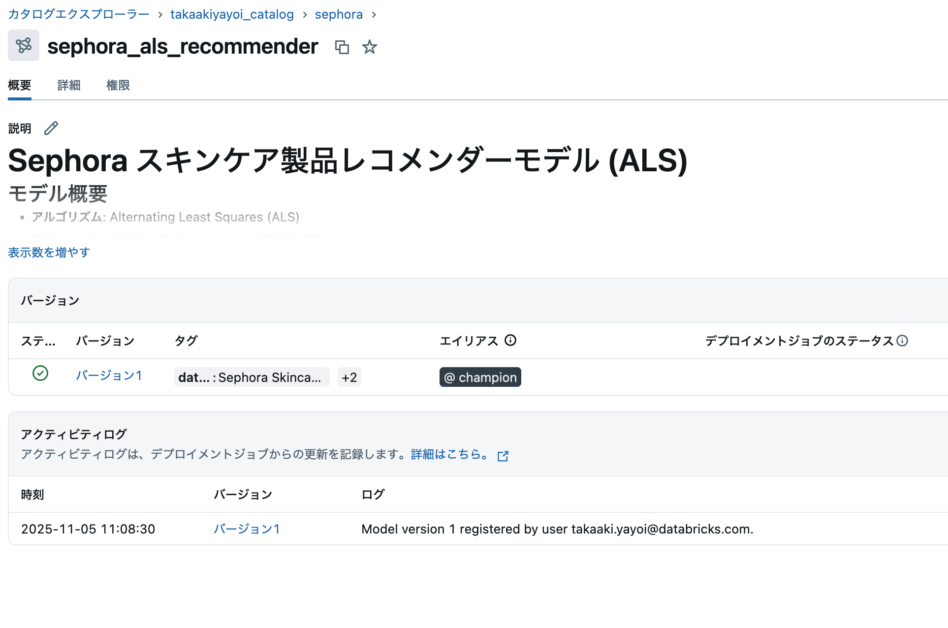
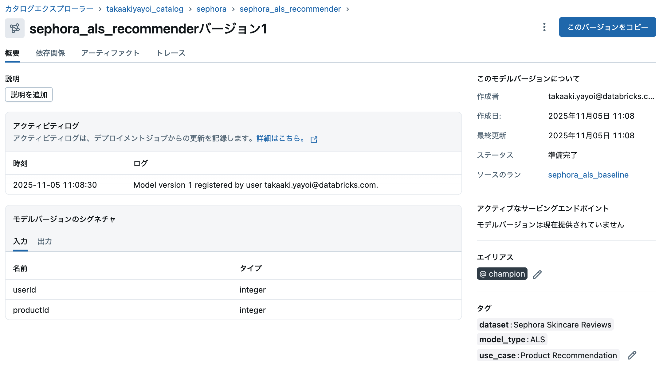
Unity Catalogでのモデル確認

左サイドバーの「Catalog」をクリック
takaakiyayoi_catalog → sephora → Models に移動
sephora_als_recommender モデルをクリック

モデルの詳細画面では以下が確認できます：

バージョン履歴: 全バージョンの一覧
メトリクス: RMSE、MAEなどの性能指標
パラメータ: モデルの設定値
リネージ: データソースとの関連
エイリアス: Champion（本番用）、Challenger（検証用）など

カタログエクスプローラでモデルが登録されていることを確認できます。

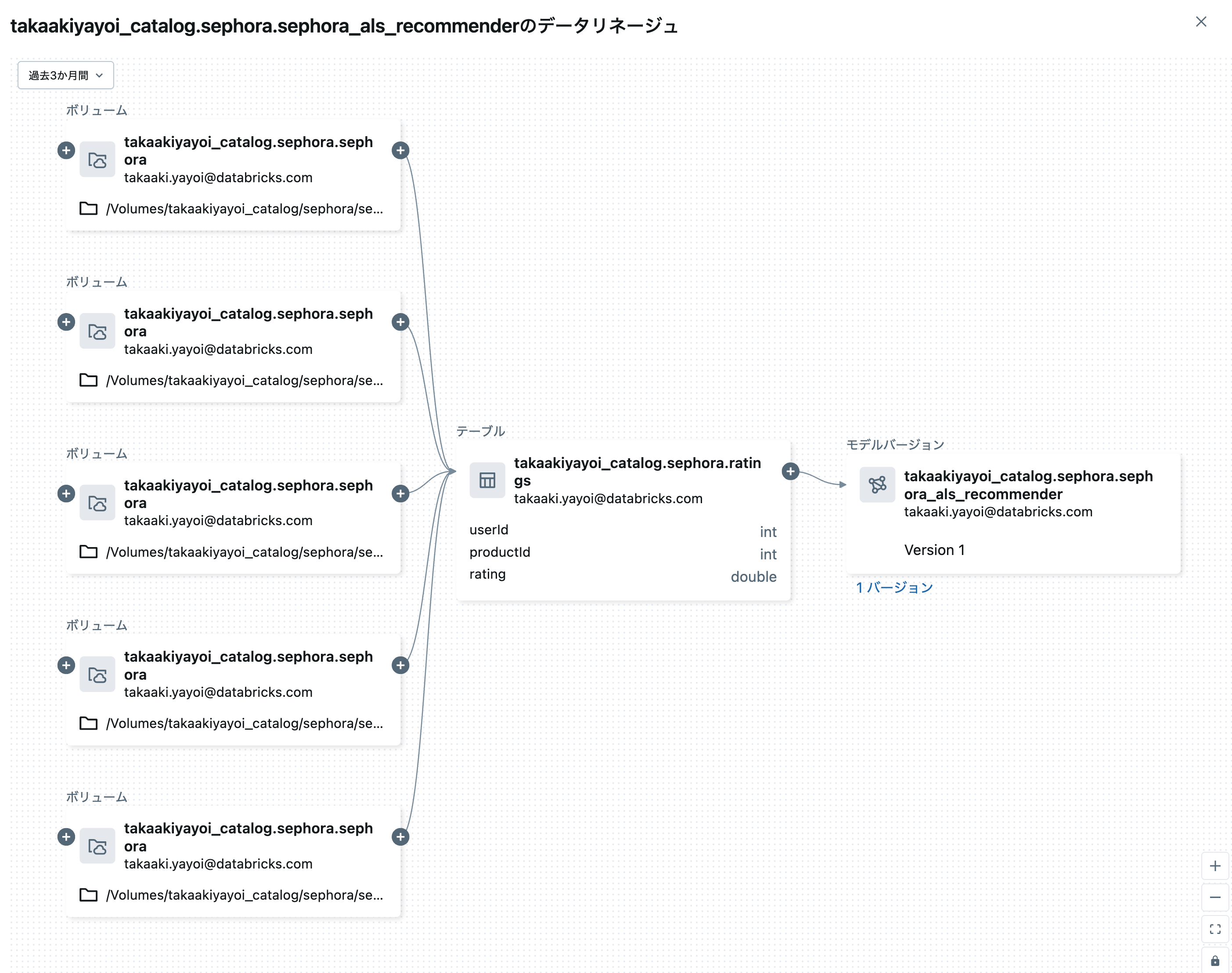
また、上のステップでリネージを設定しているので、このモデルがどのデータを用いてトレーニングされたのかを確認することができます。

モデルのロードと使用例

# Unity Catalogからモデルをロード
loaded_model = mlflow.spark.load_model(f"models:/{UC_MODEL_NAME}@Champion")

print("✓ モデルをロードしました")
print(f"  モデル名: {UC_MODEL_NAME}")
print(f"  エイリアス: Champion")

# サンプルユーザーと製品のペアを作成
sample_users = training.select("userId").distinct().limit(3).collect()
sample_products = products_indexed.select("productId").limit(10).collect()

# ユーザーと製品のペアを作成
from itertools import product as itertools_product
user_product_pairs = [
    (user[0], product[0])
    for user, product in itertools_product(sample_users, sample_products)
]

# DataFrameに変換
from pyspark.sql.types import StructType, StructField, IntegerType
schema = StructType([
    StructField("userId", IntegerType(), False),
    StructField("productId", IntegerType(), False)
])
user_product_df = spark.createDataFrame(user_product_pairs, schema)

# 予測を実行
predictions_sample = loaded_model.transform(user_product_df)

print("\n=== サンプル推薦結果 ===")
display(
    predictions_sample
    .join(products_indexed, "productId")
    .select("userId", "product_name", "brand_name", "prediction")
    .withColumnRenamed("prediction", "predicted_rating")
    .orderBy("userId", desc("predicted_rating"))
    .limit(30)
)

✓ モデルをロードしました
  モデル名: takaakiyayoi_catalog.sephora.sephora_als_recommender
  エイリアス: Champion

=== サンプル推薦結果 ===

userId	product_name	brand_name	predicted_rating
2366	7 Day Face Scrub Cream Rinse-Off Formula	CLINIQUE	2.9574928283691406
2366	Goodbye Acne Max Complexion Correction Pads	Peter Thomas Roth	2.82841157913208
2366	Grape Water Moisturizing Face Mist	Caudalie	2.513127326965332
2366	Clarifying Lotion 1	CLINIQUE	2.3645267486572266
2366	Repairwear Anti-Gravity Eye Cream	CLINIQUE	2.22860050201416
2366	Rinse-Off Foaming Cleanser	CLINIQUE	1.8009891510009766
2366	Renewing Eye Cream	Murad	1.6064350605010986
2366	All About Lips	CLINIQUE	1.280785083770752
2366	Exfoliating Face Scrub	CLINIQUE	1.2557634115219116
2366	All About Eyes Eye Cream	CLINIQUE	1.2086994647979736
13285	Repairwear Anti-Gravity Eye Cream	CLINIQUE	5.050063133239746
13285	Grape Water Moisturizing Face Mist	Caudalie	4.690354347229004
13285	Goodbye Acne Max Complexion Correction Pads	Peter Thomas Roth	4.587014198303223
13285	7 Day Face Scrub Cream Rinse-Off Formula	CLINIQUE	4.5565266609191895
13285	Rinse-Off Foaming Cleanser	CLINIQUE	4.130077362060547
13285	Exfoliating Face Scrub	CLINIQUE	4.118031024932861
13285	All About Eyes Eye Cream	CLINIQUE	3.820549726486206
13285	Clarifying Lotion 1	CLINIQUE	3.7927842140197754
13285	Renewing Eye Cream	Murad	3.564669609069824
13285	All About Lips	CLINIQUE	3.2064852714538574
17679	Clarifying Lotion 1	CLINIQUE	3.8727896213531494
17679	All About Lips	CLINIQUE	2.949568271636963
17679	Grape Water Moisturizing Face Mist	Caudalie	2.3585615158081055
17679	Goodbye Acne Max Complexion Correction Pads	Peter Thomas Roth	2.3345608711242676
17679	Rinse-Off Foaming Cleanser	CLINIQUE	2.0911519527435303
17679	Repairwear Anti-Gravity Eye Cream	CLINIQUE	1.923648476600647
17679	All About Eyes Eye Cream	CLINIQUE	1.9038817882537842
17679	Exfoliating Face Scrub	CLINIQUE	1.6859986782073975
17679	Renewing Eye Cream	Murad	1.5239790678024292
17679	7 Day Face Scrub Cream Rinse-Off Formula	CLINIQUE	1.125195026397705

9. まとめ

このノートブックでは、以下を実施しました:

データ準備: Unity Catalogテーブルからのデータ読み込み（110万レビュー、8,500製品）
探索的分析: SQL・Pythonによる製品タイプ、ブランド、価格帯の分析
モデリング: ALSアルゴリズムを使用したスキンケア製品レコメンダーの構築
評価: RMSE・MAEによるモデル性能の評価と可視化
推薦生成: ユーザーへのトップ10製品推薦と多様性分析
MLflow統合: 実験管理、モデルの自動記録、データリネージ
Unity Catalogモデル登録: モデルのバージョン管理とガバナンス

作成されたアセット

Unity Catalogテーブル: takaakiyayoi_catalog.sephora.*
登録済みモデル: takaakiyayoi_catalog.sephora.sephora_als_recommender
MLflow Experiment: /Users/takaaki.yayoi@databricks.com/20251104_sephora_als/sephora_recommender_experiment

次のステップ

Databricks SQLダッシュボード: 推薦結果とビジネスメトリクスの可視化
Genie: 自然言語でのデータ分析とインサイト抽出
Model Serving: リアルタイム推薦APIの構築とデプロイ
ハイパーパラメータチューニング: グリッドサーチで精度向上
ユーザー属性活用: 肌タイプなどを考慮したハイブリッド推薦
A/Bテスト: 推薦アルゴリズムの効果測定

はじめてのDatabricks

Databricks無料トライアル

You get articles that match your needs
You can efficiently read back useful information
You can use dark theme

What you can do with signing up