気づいたらサーバレスGPUのサンプルノートブックが増えてました。
コンピュータビジョンタスクのDETR(Detection Transformer)を使用した物体検出を試してみます。
翻訳しつつも動かなかったところは適宜修正しています。
サーバーレスGPUコンピュート: DETRオブジェクト検出カスタムファインチューニング - シングルGPUデモ
このノートブックは、Hugging Faceのサンプルを使ってA10 GPU 1台でオブジェクト検出モデルをトレーニングする方法を示します。続行するために環境パネルでパッケージ依存関係を設定する必要はありません。
このノートブックでは以下の手順を説明します:
- 依存関係のインストール
- データセットの読み込み
- データセットからのデータポイントの可視化
- データの前処理
- モデルのファインチューニング
- モデル性能の評価
- 推論の実行
- モデルをMLflowに保存
注意事項:
- このデモではA10を1台のみ使用してください。
- A10の起動には最大8分かかる場合があります。
- ノートブックはリソースに接続されるとすぐに利用可能なコンピュートを使い始めます。
- 60分間操作がないと自動的に切断されます。
- ノートブックデバッグガイドおよびSpark Connect UDFは現時点では非対応です
ステップ1) ノートブックの設定
このノートブックをコンピュートに接続しデモを実行する前に、上部のウィジェット変数を設定してください。これにより、下記のノートブックセルがカスタマイズした情報で正しく動作します:
-
experiment: トレーニング実行の出力(メトリクスやチェックポイント)が保存されるMLflow実験のパス
ステップ2) ノートブックをA10ノードに接続
- 右側パネルの「Environment」設定に移動
- 「Accelerator」をA10に設定
- 右上の「Connect」を選択し「Serverless」を選択
- すでに「Serverless」と表示されている場合は:
- 「Serverless」を選択
- 「Serverless」にカーソルを合わせる
- 「Reset」を選択
- これでノートブックは自動的にA10G GPUプールに接続されます。
ステップ3) デモノートブックを実行
- 各マークダウンセルを確認しながらデモを進めてください
- 各トレーニング用セルを実行し、A10Gでのトレーニングの様子を確認してください
シングルGPUによるDETR(DEtection TRansformer)を用いたオブジェクト検出カスタムファインチューニング
オブジェクト検出は、画像内の人間、建物、車などのインスタンスを検出するコンピュータビジョンタスクです。オブジェクト検出モデルは画像を入力として受け取り、検出されたオブジェクトのバウンディングボックスの座標とラベルを出力します。1つの画像には複数のオブジェクトが含まれる場合があり、それぞれにバウンディングボックスとラベルがあります(例:車と建物が同時に写っている)。また、同じ種類のオブジェクトが画像内の異なる場所に複数存在することもあります(例:複数の車)。このタスクは自動運転における歩行者、標識、信号機の検出などでよく使われます。他にも画像内の物体数カウントや画像検索など多くの用途があります。
このガイドは主にHuggingFaceの既存ノートブックを参考にしています。ここではDETR(畳み込みバックボーンとエンコーダ・デコーダ型トランスフォーマーを組み合わせたモデル)をCPPE-5データセットでファインチューニングし、ファインチューニング済みモデルで推論する方法を学びます。
このチュートリアルで扱う主なモデルアーキテクチャ:
手順
以下のコードで次の流れを体験できます:
- 依存関係のインストール
- CPPE-5データセットの読み込み
- データの前処理
- DETRモデルのファインチューニング
- モデル性能の評価
- 推論の実行
- MLflowへのモデル登録
us-west-2 または us-east-1 のワークスペースでサーバレスGPUを選択します。
1) 依存関係のインストール
まず、必要なライブラリをすべてインストールし、環境を整えましょう。
%pip install datasets transformers==4.43.4 evaluate==0.4.3 timm==1.0.11 albumentations==1.4.21 pydantic==2.9.2 pycocotools==2.0.8
%pip install accelerate==1.0.1
# Hugging Faceの認証が必要な場合は、以下を実行してください

# from huggingface_hub import notebook_login
# notebook_login()

import os

os.environ["HF_DATASETS_CACHE"] = "/tmp/"
os.environ["WANDB_MODE"] = "disabled"
2) CPPE-5データセットの読み込み
次に、必要なデータセットを読み込みます。CPPE-5データセットには、COVID-19パンデミックの文脈で医療用個人防護具(PPE)を特定する注釈付き画像が含まれています。まずはデータセットを読み込みましょう:
from datasets import load_dataset

cppe5 = load_dataset("cppe-5")
このデータセットには、1000枚の画像を含むトレーニングセットと29枚の画像を含むテストセットがすでに含まれています。データに慣れるために、サンプルがどのようなものか見てみましょう:
cppe5["train"][0]
{'image_id': 15,
 'image': <PIL.Image.Image image mode=RGB size=943x663>,
 'width': 943,
 'height': 663,
 'objects': {'id': [114, 115, 116, 117],
  'area': [3796, 1596, 152768, 81002],
  'bbox': [[302.0, 109.0, 73.0, 52.0],
   [810.0, 100.0, 57.0, 28.0],
   [160.0, 31.0, 248.0, 616.0],
   [741.0, 68.0, 202.0, 401.0]],
  'category': [4, 4, 0, 0]}}
データセットのサンプルには以下のフィールドがあります:
-
image_id: 画像のID -
image: 画像を含むPIL.Image.Imageオブジェクト -
width: 画像の幅 -
height: 画像の高さ -
objects: 画像内オブジェクトのバウンディングボックス情報を含む辞書:-
id: アノテーションID -
area: バウンディングボックスの面積 -
bbox: オブジェクトのバウンディングボックス(COCOフォーマット) -
category: オブジェクトのカテゴリ。Coverall (0),Face_Shield (1),Gloves (2),Goggles (3),Mask (4)など
-
bboxフィールドはDETRモデルが期待するCOCOフォーマットですが、objects内のフィールドのグルーピングがDETRのアノテーション形式と異なります。
トレーニングに使う前に前処理が必要です。
さらにデータを理解するため、サンプル画像を可視化してみましょう:
import numpy as np
import os
from PIL import Image, ImageDraw

image = cppe5["train"][0]["image"]
annotations = cppe5["train"][0]["objects"]
draw = ImageDraw.Draw(image)

categories = cppe5["train"].features["objects"]["category"].feature.names

id2label = {index: x for index, x in enumerate(categories, start=0)}
label2id = {v: k for k, v in id2label.items()}

for i in range(len(annotations["id"])):
    box = annotations["bbox"][i]
    class_idx = annotations["category"][i]
    x, y, w, h = tuple(box)
    draw.rectangle((x, y, x + w, y + h), outline="red", width=1)
    draw.text((x, y), id2label[class_idx], fill="white")

image
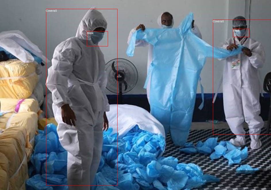
バウンディングボックスとラベルを可視化するには、データセットのメタデータ(特にcategoryフィールド)からラベルを取得します。
また、ラベルIDからラベルクラスへのマップ(id2label)とその逆(label2id)も作成しておくと便利です。
これらは後でモデルのセットアップ時にも使います。これらのマップを含めておくことで、Hugging Face Hubで他の人とモデルを共有する際にも再利用しやすくなります。
最後に、データに潜む問題を探してみましょう。オブジェクト検出用データセットでよくある問題は、画像の端を超えてしまうバウンディングボックスです。こうした"はみ出し"バウンディングボックスはトレーニング時にエラーの原因となるため、この段階で除去しておきます。このデータセットにもいくつかそのような例があります。
このガイドでは簡単のため、該当画像をデータから除外します。
remove_idx = [590, 821, 822, 875, 876, 878, 879]
keep = [i for i in range(len(cppe5["train"])) if i not in remove_idx]
cppe5["train"] = cppe5["train"].select(keep)
3) データの前処理
モデルをファインチューニングするには、事前学習済みモデルで使われた手法と正確に一致するようにデータを前処理する必要があります。
AutoImageProcessorは、画像データをpixel_values、pixel_mask、labelsに変換し、DETRモデルでトレーニングできるようにします。イメージプロセッサには以下の属性があります:
image_mean = [0.485, 0.456, 0.406 ]image_std = [0.229, 0.224, 0.225]
これらはモデルの事前学習時に画像を正規化するために使われた平均値と標準偏差です。推論やファインチューニング時にもこれらの値を再現することが重要です。
次に、ファインチューニングしたいモデルと同じチェックポイントからイメージプロセッサをインスタンス化しましょう:
from transformers import AutoImageProcessor

checkpoint = "facebook/detr-resnet-50"
image_processor = AutoImageProcessor.from_pretrained(checkpoint)
画像をimage_processorに渡す前に、データセットに2つの前処理変換を適用します:
- 画像の拡張(オーグメンテーション)
- アノテーションをDETRの期待する形式に変換
まず、モデルがトレーニングデータに過学習しないよう、データ拡張を行います。ここではAlbumentationsを使います。このライブラリは画像とバウンディングボックスの両方に変換を適用できます。🤗 Datasetsの公式ガイドでも同じデータセットを例にしています。ここでも同様に、各画像を(480, 480)にリサイズし、左右反転、明るさ調整を行います:
import albumentations
import numpy as np
import torch

# Albumentationsによる画像拡張とバウンディングボックス変換
transform = albumentations.Compose(
    [
        albumentations.Resize(480, 480),
        albumentations.HorizontalFlip(p=1.0),
        albumentations.RandomBrightnessContrast(p=1.0),
    ],
    bbox_params=albumentations.BboxParams(format="coco", label_fields=["category"]),
)
image_processorはアノテーションが次の形式であることを期待します: {'image_id': int, 'annotations': List[Dict]}
各辞書はCOCOオブジェクトアノテーションです。1つのサンプルのアノテーションを変換する関数を追加しましょう:
def formatted_anns(image_id, category, area, bbox):
    annotations = []
    for i in range(0, len(category)):
        new_ann = {
            "image_id": image_id,
            "category_id": category[i],
            "isCrowd": 0,  # COCO形式のisCrowdフラグ
            "area": area[i],
            "bbox": list(bbox[i]),
        }
        annotations.append(new_ann)

    return annotations
次に、画像とアノテーションの変換を組み合わせてバッチに適用できるようにします:
# バッチ変換用の関数
def transform_aug_ann(examples):
    image_ids = examples["image_id"]
    images, bboxes, area, categories = [], [], [], []
    for image, objects in zip(examples["image"], examples["objects"]):
        image = np.array(image.convert("RGB"))[:, :, ::-1]
        out = transform(
            image=image, bboxes=objects["bbox"], category=objects["category"]
        )

        area.append(objects["area"])
        images.append(out["image"])
        bboxes.append(out["bboxes"])
        categories.append(out["category"])

    targets = [
        {"image_id": id_, "annotations": formatted_anns(id_, cat_, ar_, box_)}
        for id_, cat_, ar_, box_ in zip(image_ids, categories, area, bboxes)
    ]

    return image_processor(images=images, annotations=targets, return_tensors="pt")
with_transformメソッドを使って、データセット全体にこの前処理関数を適用します。このメソッドはデータセットの要素を読み込む際にオンザフライで変換を適用します。
この時点で、変換後のデータセットのサンプルがどのようになっているか確認できます。pixel_valuesのテンソル、pixel_maskのテンソル、labelsが含まれているはずです。
cppe5["train"] = cppe5["train"].with_transform(transform_aug_ann)
cppe5["train"][15]
The `max_size` parameter is deprecated and will be removed in v4.26. Please specify in `size['longest_edge'] instead`.
{'pixel_values': tensor([[[ 1.3584,  1.3584,  1.3584,  ..., -1.6898, -1.6898, -1.6898],
          [ 1.3584,  1.3584,  1.3584,  ..., -1.6898, -1.6898, -1.6898],
          [ 1.3584,  1.3584,  1.3584,  ..., -1.6727, -1.6727, -1.6727],
          ...,
          [-1.2617, -1.2617, -1.2617,  ..., -1.7069, -1.7069, -1.7069],
          [-1.2445, -1.2445, -1.2445,  ..., -1.7069, -1.6898, -1.6898],
          [-1.2445, -1.2445, -1.2445,  ..., -1.7069, -1.6898, -1.6898]],

         [[ 1.7983,  1.7983,  1.7983,  ..., -1.5455, -1.5455, -1.5455],
          [ 1.7983,  1.7983,  1.7983,  ..., -1.5455, -1.5455, -1.5455],
          [ 1.7983,  1.7983,  1.7983,  ..., -1.5280, -1.5280, -1.5280],
          ...,
          [-0.9853, -0.9853, -0.9853,  ..., -1.5630, -1.5630, -1.5630],
          [-0.9678, -0.9678, -0.9678,  ..., -1.5630, -1.5455, -1.5455],
          [-0.9678, -0.9678, -0.9678,  ..., -1.5630, -1.5455, -1.5455]],

         [[ 1.8905,  1.8905,  1.8905,  ..., -1.3513, -1.3513, -1.3513],
          [ 1.8905,  1.8905,  1.8905,  ..., -1.3513, -1.3513, -1.3513],
          [ 1.8905,  1.8905,  1.8905,  ..., -1.3339, -1.3339, -1.3339],
          ...,
          [-0.6715, -0.6715, -0.6715,  ..., -1.2467, -1.2467, -1.2467],
          [-0.6541, -0.6541, -0.6541,  ..., -1.2467, -1.2293, -1.2293],
          [-0.6541, -0.6541, -0.6541,  ..., -1.2467, -1.2293, -1.2293]]]),
 'pixel_mask': tensor([[1, 1, 1,  ..., 1, 1, 1],
         [1, 1, 1,  ..., 1, 1, 1],
         [1, 1, 1,  ..., 1, 1, 1],
         ...,
         [1, 1, 1,  ..., 1, 1, 1],
         [1, 1, 1,  ..., 1, 1, 1],
         [1, 1, 1,  ..., 1, 1, 1]]),
 'labels': {'size': tensor([800, 800]), 'image_id': tensor([756]), 'class_labels': tensor([4]), 'boxes': tensor([[0.7340, 0.6986, 0.3414, 0.5944]]), 'area': tensor([519544.4375]), 'iscrowd': tensor([0]), 'orig_size': tensor([480, 480])}}
個々の画像の拡張とアノテーションの準備ができましたが、前処理はまだ完了していません。最後のステップとして、画像をバッチ化するためのカスタムcollate_fnを作成します。
画像(pixel_values)をバッチ内で最大サイズにパディングし、どのピクセルが実データ(1)でどれがパディング(0)かを示すpixel_maskも作成します。
# DataLoader用のカスタムcollate関数

def collate_fn(batch):
    pixel_values = [item["pixel_values"] for item in batch]
    encoding = image_processor.pad(pixel_values, return_tensors="pt")
    labels = [item["labels"] for item in batch]
    batch = {}
    batch["pixel_values"] = encoding["pixel_values"]
    batch["pixel_mask"] = encoding["pixel_mask"]
    batch["labels"] = labels
    return batch
4) DETRモデルのファインチューニング
前のセクションでほとんどの準備ができたので、いよいよモデルのトレーニングに進みます!
このデータセットの画像はリサイズ後もかなり大きいため、ファインチューニングには少なくとも1つのGPUが必要です。
トレーニングの流れ:
- AutoModelForObjectDetectionでモデルを読み込みます(前処理と同じチェックポイントを使用)。
- TrainingArgumentsでハイパーパラメータを定義します。
- モデル、データセット、イメージプロセッサ、データコレータとともにTrainerに渡します。
- train()を呼び出してモデルをファインチューニングします。
モデルを読み込む際は、先ほど作成したlabel2idとid2labelのマップも渡します。また、ignore_mismatched_sizes=Trueを指定して既存の分類ヘッドを新しいものに置き換えます。
from transformers import AutoModelForObjectDetection

# 事前学習済みモデルをid2label/label2idマップ付きで読み込む
model = AutoModelForObjectDetection.from_pretrained(
    checkpoint,
    id2label=id2label,
    label2id=label2id,
    ignore_mismatched_sizes=True,
)
device = "cuda"
model = model.to(device)
TrainingArgumentsでは、output_dirでモデルの保存先を指定し、ハイパーパラメータを設定します。
未使用カラムを削除しないようにすることが重要です。これを削除すると画像カラムも消えてしまい、pixel_valuesが作れなくなります。そのためremove_unused_columnsはFalseに設定してください。
モデルをHubにアップロードしたい場合はpush_to_hubをTrueにします(Hugging Faceにサインインしている必要があります)。
# TCPストア問題の回避策として明示的にプロセスグループを初期化
import torch.distributed as dist

store = dist.FileStore("/tmp/sharedfile", world_size=1)
dist.init_process_group(
    backend="nccl",
    store=store,  # FileStoreインスタンスを渡す
    world_size=1,  # 参加プロセス数
    rank=0,  # 現在のプロセスのランク
)
from transformers import TrainingArguments

training_args = TrainingArguments(
    output_dir="detr_finetuned_cppe5",
    num_train_epochs=30,
    fp16=False,
    per_device_train_batch_size=8,
    dataloader_num_workers=4,
    learning_rate=5e-5,
    lr_scheduler_type="cosine",
    weight_decay=1e-4,
    max_grad_norm=0.01,
    logging_steps=100,
    # metric_for_best_model="eval_map",
    # greater_is_better=True,
    # load_best_model_at_end=True,
    # eval_strategy="epoch",
    # save_strategy="epoch",
    # save_total_limit=2,
    remove_unused_columns=False,
    # eval_do_concat_batches=False,
    # push_to_hub=True,
    report_to=[],
)
最後にすべてをまとめて、train()を呼び出します:
from transformers import Trainer

trainer = Trainer(
    model=model,
    args=training_args,
    data_collator=collate_fn,
    train_dataset=cppe5["train"],
    tokenizer=image_processor,
)

trainer.train()
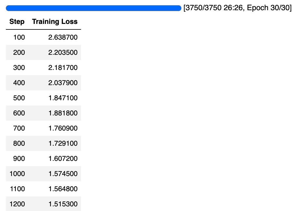
TrainOutput(global_step=3750, training_loss=1.4090041809082032, metrics={'train_runtime': 1604.1884, 'train_samples_per_second': 18.57, 'train_steps_per_second': 2.338, 'total_flos': 1.42341326915328e+19, 'train_loss': 1.4090041809082032, 'epoch': 30.0})
5) モデル性能の評価
オブジェクト検出モデルは一般的にCOCOスタイルのメトリクスで評価されます。
既存のメトリクス実装を使うこともできますが、ここではtorchvisionの評価器を使って、Hubにアップロードした最終モデルを評価します。
torchvisionの評価器を使うには、COCO形式の正解データセットを用意する必要があります。COCOデータセットAPIは特定の形式でデータが保存されていることを要求するため、まず画像とアノテーションをディスクに保存します。トレーニング時と同様に、cppe5["test"]のアノテーションを整形しますが、画像自体はそのまま使います。
評価ステップは大きく3つに分けられます。
まず、cppe5["test"]セットを準備します: アノテーションを整形し、データをディスクに保存します。
import json

# トレーニング時と同じ形式でアノテーションを整形(データ拡張は不要)
def val_formatted_anns(image_id, objects):
    annotations = []
    for i in range(0, len(objects["id"])):
        new_ann = {
            "id": objects["id"][i],
            "category_id": objects["category"][i],
            "iscrowd": 0,  # COCO形式のisCrowdフラグ
            "image_id": image_id,
            "area": objects["area"][i],
            "bbox": objects["bbox"][i],
        }
        annotations.append(new_ann)

    return annotations

# torchvision.datasets.CocoDetectionが期待するファイルに画像とアノテーションを保存

def save_cppe5_annotation_file_images(cppe5):
    output_json = {}
    path_output_cppe5 = f"{os.getcwd()}/cppe5/"

    if not os.path.exists(path_output_cppe5):
        os.makedirs(path_output_cppe5)

    path_anno = os.path.join(path_output_cppe5, "cppe5_ann.json")
    categories_json = [
        {"supercategory": "none", "id": id, "name": id2label[id]} for id in id2label
    ]
    output_json["images"] = []
    output_json["annotations"] = []
    for example in cppe5:
        ann = val_formatted_anns(example["image_id"], example["objects"])
        output_json["images"].append(
            {
                "id": example["image_id"],
                "width": example["image"].width,
                "height": example["image"].height,
                "file_name": f"{example['image_id']}.png",
            }
        )
        output_json["annotations"].extend(ann)
    output_json["categories"] = categories_json

    with open(path_anno, "w") as file:
        json.dump(output_json, file, ensure_ascii=False, indent=4)

    for im, img_id in zip(cppe5["image"], cppe5["image_id"]):
        path_img = os.path.join(path_output_cppe5, f"{img_id}.png")
        im.save(path_img)

    return path_output_cppe5, path_anno
次に、cocoevaluatorで使えるCocoDetectionクラスのインスタンスを準備します。
import torchvision

# COCO評価用のCocoDetectionクラスを拡張
class CocoDetection(torchvision.datasets.CocoDetection):
    def __init__(self, img_folder, feature_extractor, ann_file):
        super().__init__(img_folder, ann_file)
        self.feature_extractor = feature_extractor

    def __getitem__(self, idx):
        # PIL画像とCOCO形式ターゲットを読み込む
        img, target = super(CocoDetection, self).__getitem__(idx)

        # 画像とターゲットをDETR形式に変換し、リサイズ・正規化
        image_id = self.ids[idx]
        target = {"image_id": image_id, "annotations": target}
        encoding = self.feature_extractor(
            images=img, annotations=target, return_tensors="pt"
        )
        pixel_values = encoding["pixel_values"].squeeze()  # バッチ次元を除去
        target = encoding["labels"][0]  # バッチ次元を除去

        return {"pixel_values": pixel_values, "labels": target}

path_output_cppe5, path_anno = save_cppe5_annotation_file_images(cppe5["test"])
test_ds_coco_format = CocoDetection(path_output_cppe5, image_processor, path_anno)
loading annotations into memory...
Done (t=0.05s)
creating index...
index created!
最後に、メトリクスを読み込み、評価を実行します。
import evaluate
from tqdm import tqdm

module = evaluate.load("ybelkada/cocoevaluate", coco=test_ds_coco_format.coco)
val_dataloader = torch.utils.data.DataLoader(
    test_ds_coco_format,
    batch_size=8,
    shuffle=False,
    num_workers=4,
    collate_fn=collate_fn,
)
with torch.no_grad():
    for idx, batch in enumerate(tqdm(val_dataloader)):
        pixel_values = batch["pixel_values"].to(device)
        pixel_mask = batch["pixel_mask"].to(device)

        labels = [
            {k: v for k, v in t.items()} for t in batch["labels"]
        ]  # DETR形式でリサイズ・正規化済み

        # 順伝播
        outputs = model(pixel_values=pixel_values, pixel_mask=pixel_mask)

        orig_target_sizes = torch.stack(
            [target["orig_size"] for target in labels], dim=0
        )
        results = image_processor.post_process(
            outputs, orig_target_sizes
        )  # モデル出力をCOCO API形式に変換

        module.add(prediction=results, reference=labels)
        del batch

results = module.compute()
print(results)
  0%|          | 0/4 [00:00<?, ?it/s]`post_process` is deprecated and will be removed in v5 of Transformers, please use `post_process_object_detection` instead, with `threshold=0.` for equivalent results.
100%|██████████| 4/4 [00:04<00:00,  1.13s/it]
Accumulating evaluation results...
DONE (t=0.04s).
IoU metric: bbox
 Average Precision  (AP) @[ IoU=0.50:0.95 | area=   all | maxDets=100 ] = 0.190
 Average Precision  (AP) @[ IoU=0.50      | area=   all | maxDets=100 ] = 0.434
 Average Precision  (AP) @[ IoU=0.75      | area=   all | maxDets=100 ] = 0.147
 Average Precision  (AP) @[ IoU=0.50:0.95 | area= small | maxDets=100 ] = 0.106
 Average Precision  (AP) @[ IoU=0.50:0.95 | area=medium | maxDets=100 ] = 0.078
 Average Precision  (AP) @[ IoU=0.50:0.95 | area= large | maxDets=100 ] = 0.257
 Average Recall     (AR) @[ IoU=0.50:0.95 | area=   all | maxDets=  1 ] = 0.201
 Average Recall     (AR) @[ IoU=0.50:0.95 | area=   all | maxDets= 10 ] = 0.343
 Average Recall     (AR) @[ IoU=0.50:0.95 | area=   all | maxDets=100 ] = 0.364
 Average Recall     (AR) @[ IoU=0.50:0.95 | area= small | maxDets=100 ] = 0.106
 Average Recall     (AR) @[ IoU=0.50:0.95 | area=medium | maxDets=100 ] = 0.173
 Average Recall     (AR) @[ IoU=0.50:0.95 | area= large | maxDets=100 ] = 0.467
{'iou_bbox': {'AP-IoU=0.50:0.95-area=all-maxDets=100': 0.18986616880884727, 'AP-IoU=0.50-area=all-maxDets=100': 0.434433914124076, 'AP-IoU=0.75-area=all-maxDets=100': 0.14696182612538788, 'AP-IoU=0.50:0.95-area=small-maxDets=100': 0.1062234794908062, 'AP-IoU=0.50:0.95-area=medium-maxDets=100': 0.07756245650991515, 'AP-IoU=0.50:0.95-area=large-maxDets=100': 0.2569967644957088, 'AR-IoU=0.50:0.95-area=all-maxDets=1': 0.2014579799553281, 'AR-IoU=0.50:0.95-area=all-maxDets=10': 0.34262974639204147, 'AR-IoU=0.50:0.95-area=all-maxDets=100': 0.36387600965144357, 'AR-IoU=0.50:0.95-area=small-maxDets=100': 0.10598290598290598, 'AR-IoU=0.50:0.95-area=medium-maxDets=100': 0.1733391304347826, 'AR-IoU=0.50:0.95-area=large-maxDets=100': 0.46712842712842717}}
これらの結果はTrainingArgumentsのハイパーパラメータを調整することでさらに改善できます。ぜひ試してみてください!
6) 推論の実行
DETRモデルのファインチューニング、評価、Hugging Face Hubへのアップロードが完了したので、推論にも使えます。
最も簡単な方法はPipelineを使うことです。
オブジェクト検出用のパイプラインをインスタンス化し、画像を渡してみましょう:
cppe5
DatasetDict({
    train: Dataset({
        features: ['image_id', 'image', 'width', 'height', 'objects'],
        num_rows: 993
    })
    test: Dataset({
        features: ['image_id', 'image', 'width', 'height', 'objects'],
        num_rows: 29
    })
})
from transformers import pipeline
import requests
from io import BytesIO

image = cppe5["test"][22]["image"]

# オブジェクト検出パイプラインを作成
obj_detector = pipeline(
    "object-detection", model=model, image_processor=image_processor
)
obj_detector(image)
Hardware accelerator e.g. GPU is available in the environment, but no `device` argument is passed to the `Pipeline` object. Model will be on CPU.
[{'score': 0.9396964311599731,
  'label': 'Mask',
  'box': {'xmin': 806, 'ymin': 354, 'xmax': 1180, 'ymax': 676}},
 {'score': 0.701697826385498,
  'label': 'Coverall',
  'box': {'xmin': 17, 'ymin': 11, 'xmax': 1976, 'ymax': 1111}},
 {'score': 0.5664281249046326,
  'label': 'Coverall',
  'box': {'xmin': 1, 'ymin': 267, 'xmax': 597, 'ymax': 1107}}]
パイプラインの結果を手動で再現することもできます:
with torch.no_grad():
    inputs = image_processor(images=image, return_tensors="pt").to("cuda:0")
    # 入力テンソルを確認したい場合はprint(inputs)
    outputs = model(**inputs)
    target_sizes = torch.tensor([image.size[::-1]])
    results = image_processor.post_process_object_detection(
        outputs, threshold=0.5, target_sizes=target_sizes
    )[0]

for score, label, box in zip(results["scores"], results["labels"], results["boxes"]):
    box = [round(i, 2) for i in box.tolist()]
    print(
        f"{model.config.id2label[label.item()]}を信頼度{round(score.item(), 3)}で検出 場所: {box}"
    )
Maskを信頼度0.958で検出 場所: [808.98, 349.91, 1179.63, 673.04]
Coverallを信頼度0.697で検出 場所: [26.26, 22.07, 1959.08, 1108.05]
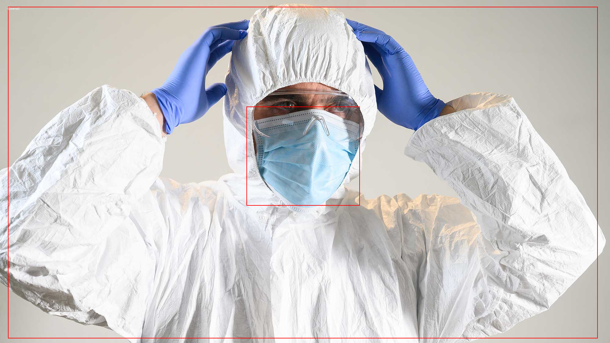
結果をプロットしてみましょう:
draw = ImageDraw.Draw(image)

for score, label, box in zip(results["scores"], results["labels"], results["boxes"]):
    box = [round(i, 2) for i in box.tolist()]
    x, y, x2, y2 = tuple(box)
    draw.rectangle((x, y, x2, y2), outline="red", width=2)
    draw.text((x, y), model.config.id2label[label.item()], fill="white")

# 画像を表示
image
7) モデルをMLflowに登録してサービング
dbutils.widgets.text("experiment", "/Users/{username}/object-detection-demo") # MLflow実験パス用ウィジェット
import mlflow

# ユーザー名を取得し、MLflow実験パスを作成
username = (
    dbutils.notebook.entry_point.getDbutils().notebook().getContext().userName().get()
)
experiment_path = f'/Users/{username}/{dbutils.widgets.get("experiment")}'
experiment = mlflow.set_experiment(experiment_path)

# モデルをMLflowに記録
model_info = mlflow.transformers.log_model(obj_detector, artifact_path="artifacts")
print(model_info.model_uri) # モデルURIを表示
runs:/76fbace47acd419a8f53d8f22abf1f3e/artifacts
detector = mlflow.transformers.load_model(model_info.model_uri) # MLflowからモデルをロード
outputs = detector(image)  # 推論を実行
outputs
[{'score': 0.950192391872406,
  'label': 'Mask',
  'box': {'xmin': 802, 'ymin': 348, 'xmax': 1170, 'ymax': 655}},
 {'score': 0.6706351637840271,
  'label': 'Coverall',
  'box': {'xmin': 31, 'ymin': 33, 'xmax': 1956, 'ymax': 1101}},
 {'score': 0.5532757639884949,
  'label': 'Coverall',
  'box': {'xmin': 862, 'ymin': 279, 'xmax': 1972, 'ymax': 1100}}]