Variational Autoencoderを使った画像の異常検知 後編 （塩尻MLもくもく会＃7）

前編では、ヒートマップを使って異常個所を可視化しました。

後編では、従来手法と提案手法を数値的に比較してみます。
使うツールは、ROC曲線です。

ROC曲線

ROC曲線は、ラベル間のデータ数に差があるときに使われます。
ROC曲線について、詳しく知りたい方はこちら↓を参考にしてください。
http://www.randpy.tokyo/entry/roc_auc

今回は、ラベル間のデータ数に大きな差はありませんが、論文にならって
ROC曲線を描画します。最終的に、AUCを算出して、これが大きい方が優れた
異常検知器といえます。

コードの解説

コードの一部を解説します。

異常スコアの算出

論文によると、異常判定の基準は以下のとおりです。

このパッチ全てに関して異常度を算出し、少なくとも1枚が閾値を
超えてる場合、テストデータは異常であると判断した．

パッチというのは、前編でお伝えした小窓に相当します。
前編では、下記のヒートマップを作成するにあたり、元の画像（サイズ28×28）に
対し、小窓（サイズ8×8）を上下左右に走らせました。

このとき、1枚の画像から小窓のスコアは21×21＝441個出てきます。
論文に従うと、441個の小窓のスコアの中から、その最大値（スコアが高いほど異常度が
高いです。）をその画像の異常スコアとします。

そして、閾値を決め、閾値より異常スコアが高いものを「異常画像」、
低いものを「正常画像」と判定します。

まとめると、以下のとおりです。

1枚の画像　→　小窓を走らせる　→　441個のスコア　→　スコアの最大値　＝　異常スコア　→　閾値と比較

pythonのコードは以下のとおりです。関数には、テストデータを渡して、
小窓を走らせながら、画像1枚1枚に異常スコアを付けています。
nameの名前で、従来手法と提案手法を切り替えて評価しています。

#最大異常値の計算
def result_score(model, x, name, height=8, width=8, move=2):
    score = []

    for k in range(len(x)):
        max_score = -1000000000
        if k%100 == 0:
          print(k)

        for i in range(int((x.shape[1]-height)/move)):
            for j in range(int((x.shape[2]-width)/move)):
                x_sub = x[k, i*move:i*move+height, j*move:j*move+width, 0]
                x_sub = x_sub.reshape(1, height, width, 1)

                #従来手法
                if name == "old_":
                    #スコア
                    temp_score = model.evaluate(x_sub, batch_size=1, verbose=0)
                    if temp_score > max_score:
                        max_score = temp_score

                #提案手法
                else:
                    #スコア
                    mu, sigma = model.predict(x_sub, batch_size=1, verbose=0)
                    loss = 0
                    for o in range(height):
                        for l in range(width):
                            loss += 0.5 * (x_sub[0,o,l,0] - mu[0,o,l,0])**2 / sigma[0,o,l,0]
                    if loss > max_score:
                       max_score = loss

        score.append(max_score)

    return(score)

ROC曲線の描画

ROC曲線の描画は、以下の記事を参考にしました。
https://qiita.com/9pid/items/53946c3ec4b2489e7cb2

scikit-learnを使えば一発です。

MNISTを使った結果

※11/21修正　コードにバグがあった関係で、図と文章を全面的に修正しました。

Colaboratoryの場合、計算時間は学習で10分、テストデータの評価で２時間ほど
かかります。

ROC曲線は以下のとおりです。

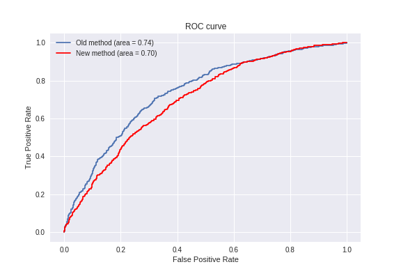
グラフの中のareaがAUCに相当します。そして、AUCが高いほうが優秀な異常検知器です。

予想に反して、従来手法の方が良い結果となりました。
提案手法の精度が落ちた理由は、後で考察します。

Fashion-MNISTを使った結果

※11/21修正　コードにバグがあった関係で、図と文章を全面的に修正しました。

計算時間はMNISTと同じくらいでした。

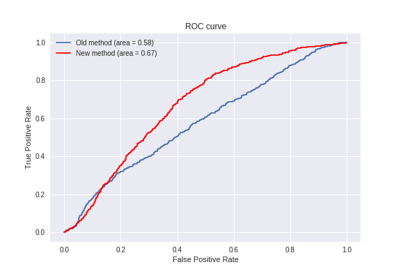
こちらはMNISTと逆で、提案手法の方が良い結果となりました。
この理由も後で考察します。

考察　11/21追記

MNISTとFashion-MNISTで結果が変わった理由を考察してみると、
MNISTでは以下の図のような学習結果になっていると思われます。

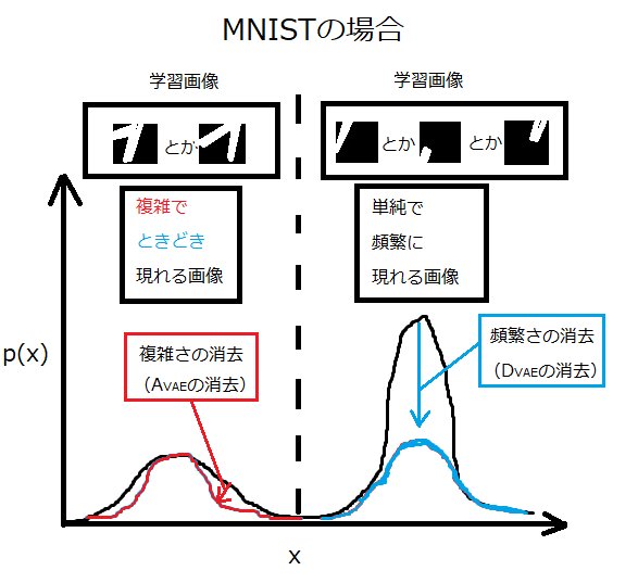
そして、テストの際に1と9を入力すると、直線部分の画像は右の山に
位置してきます。一方、異常判別の材料となる画像（1の折れ曲がり部や
9の曲線部分の画像）は左の山に位置してきます。そして、1の折れ曲
がり部は左の山の「中央」付近に、9の曲線部分は左の山の「端」に
位置することになり、異常判別ができます。

ここで重要なのは、右の山は無視して良いということです。つまり、
異常か正常かを判断する材料は左の山だけで十分です。

ところが、提案手法では右の山を下げて、左の山と同じ土俵で勝負させます。
よって、提案手法では、本来無視してよい右の山（直線部分の画像）も判別し
異常と認識してしまっている可能性が高く、精度を下げる一因になっていると
思われます。

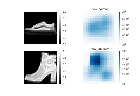
一方、Fashion-MNISTはブーツの　かかと　は複雑なため左の山に、
ブーツの口は単純なため右の山に属していると思われます。従って、
どちらの山も判断材料になるため、左右の山を同じ土俵で勝負させる
提案手法の方が精度が出たと思われます。

まとめますと、「複雑な」画像にしか異常が出ない場合は、従来手法の
方が優れていると思われます。工業製品のように「単純な」ところにも
「複雑な」ところにも異常が出る場合は、提案手法の方が優れていると
思われます。

ちなみに、Pythonでコードを組む場合、計算速度については、従来手法の方が
速く（model.evaluate()を使っているため）現場向きかと思われます。
一方、提案手法はfor文を駆使しているため、速度が遅くなります。

まとめ

※11/21修正　コードにバグがあった関係で、文章を修正しました。

前編と後編に分けて、VAEによる画像の異常検知を実装してきました。
見てお分かりのとおり、提案手法は視覚的にも能力的にも優れていること
が分かりました。

能力の面では、考察に示したとおり、異常検知の対象となる画像の性質を
考えて使い分けした方が良さそうです。

余裕があったら、本手法を使って画像以外の異常検知もやってみたいと思います。

2018/1/8追記
本手法より精度が良い論文の記事を書きました。
https://qiita.com/shinmura0/items/cfb51f66b2d172f2403b

コード全文

9/15　追記：コードにバグがありました。お詫びを申し上げ、修正させていただきます。
12/18　コード修正 （@gungiven さんご指摘ありがとうございます。）

from __future__ import absolute_import
from __future__ import division
from __future__ import print_function

from keras.layers import Lambda, Input, Dense, Reshape
from keras.models import Model
from keras.datasets import mnist
from keras.datasets import fashion_mnist
from keras.losses import mse
from keras.utils import plot_model
from keras import backend as K
from keras.layers import BatchNormalization, Activation, Flatten
from keras.layers.convolutional import Conv2DTranspose, Conv2D

import numpy as np
import matplotlib.pyplot as plt
import matplotlib.colors as colors
import os
from sklearn import metrics

#最大異常値の計算
def result_score(model, x, name, height=8, width=8, move=2):
    score = []

    for k in range(len(x)):
        max_score = -1000000000
        if k%100 == 0:
          print(k)

        for i in range(int((x.shape[1]-height)/move)+1):
            for j in range(int((x.shape[2]-width)/move)+1):
                x_sub = x[k, i*move:i*move+height, j*move:j*move+width, 0]
                x_sub = x_sub.reshape(1, height, width, 1)

                #従来手法
                if name == "old_":
                    #スコア
                    temp_score = model.evaluate(x_sub, batch_size=1, verbose=0)
                    if temp_score > max_score:
                        max_score = temp_score

                #提案手法
                else:
                    #スコア
                    mu, sigma = model.predict(x_sub, batch_size=1, verbose=0)
                    loss = 0
                    for o in range(height):
                        for l in range(width):
                            loss += 0.5 * (x_sub[0,o,l,0] - mu[0,o,l,0])**2 / sigma[0,o,l,0]
                    if loss > max_score:
                       max_score = loss

        score.append(max_score)

    return(score)

#8×8のサイズに切り出す
def cut_img(x, number, height=8, width=8):
    print("cutting images ...")
    x_out = []
    x_shape = x.shape

    for i in range(number):
        shape_0 = np.random.randint(0,x_shape[0])
        shape_1 = np.random.randint(0,x_shape[1]-height)
        shape_2 = np.random.randint(0,x_shape[2]-width)
        temp = x[shape_0, shape_1:shape_1+height, shape_2:shape_2+width, 0]
        x_out.append(temp.reshape((height, width, x_shape[3])))

    print("Complete.")
    x_out = np.array(x_out)

    return x_out

# reparameterization trick
# instead of sampling from Q(z|X), sample eps = N(0,I)
# z = z_mean + sqrt(var)*eps
def sampling(args):
    z_mean, z_log_var = args
    batch = K.shape(z_mean)[0]
    dim = K.int_shape(z_mean)[1]
    # by default, random_normal has mean=0 and std=1.0
    epsilon = K.random_normal(shape=(batch, dim))
    return z_mean + K.exp(0.5 * z_log_var) * epsilon

# dataset
(x_train, y_train), (x_test, y_test) = mnist.load_data()
#(x_train, y_train), (x_test, y_test) = fashion_mnist.load_data()

x_train = x_train.reshape(x_train.shape[0], 28, 28, 1)
x_test = x_test.reshape(x_test.shape[0], 28, 28, 1)

x_train = x_train.astype('float32') / 255
x_test = x_test.astype('float32') / 255

#1と9のデータ抽出
x_train_1 = []
x_test_1 = []
x_test_9 = []

x_train_shape = x_train.shape

for i in range(len(x_train)):
  if y_train[i] == 1:#スニーカーは7
    temp = x_train[i,:,:,:]
    x_train_1.append(temp.reshape((x_train_shape[1],x_train_shape[2],x_train_shape[3])))

x_train_1 = np.array(x_train_1)
x_train_1 = cut_img(x_train_1, 100000)
print("train data:",len(x_train_1))

for i in range(len(x_test)):
  if y_test[i] == 1:#スニーカーは7
    temp = x_test[i,:,:,:]
    x_test_1.append(temp.reshape((x_train_shape[1],x_train_shape[2],x_train_shape[3])))

  if y_test[i] == 9:
    temp = x_test[i,:,:,:]
    x_test_9.append(temp.reshape((x_train_shape[1],x_train_shape[2],x_train_shape[3])))

x_test_1 = np.array(x_test_1)
x_test_9 = np.array(x_test_9)

# network parameters
input_shape=(8, 8, 1)
batch_size = 128
latent_dim = 2
epochs = 10
Nc = 16

# build encoder model
inputs = Input(shape=input_shape, name='encoder_input')
x = Conv2D(Nc, kernel_size=2, strides=2)(inputs)
x = BatchNormalization()(x)
x = Activation('relu')(x)
x = Conv2D(2*Nc, kernel_size=2, strides=2)(x)
x = BatchNormalization()(x)
x = Activation('relu')(x)
x = Flatten()(x)

z_mean = Dense(latent_dim, name='z_mean')(x)
z_log_var = Dense(latent_dim, name='z_log_var')(x)
z = Lambda(sampling, output_shape=(latent_dim,), name='z')([z_mean, z_log_var])

encoder = Model(inputs, [z_mean, z_log_var, z], name='encoder')
#encoder.summary()

# build decoder model
latent_inputs = Input(shape=(latent_dim,), name='z_sampling')
x = Dense(2*2)(latent_inputs)
x = BatchNormalization()(x)
x = Activation('relu')(x)
x = Reshape((2,2,1))(x)
x = Conv2DTranspose(2*Nc, kernel_size=2, strides=2, padding='same')(x)
x = BatchNormalization()(x)
x = Activation('relu')(x)
x = Conv2DTranspose(Nc, kernel_size=2, strides=2, padding='same')(x)
x = BatchNormalization()(x)
x = Activation('relu')(x)

x1 = Conv2DTranspose(1, kernel_size=4, padding='same')(x)
x1 = BatchNormalization()(x1)
out1 = Activation('sigmoid')(x1)#out.shape=(n,28,28,1)

x2 = Conv2DTranspose(1, kernel_size=4, padding='same')(x)
x2 = BatchNormalization()(x2)
out2 = Activation('sigmoid')(x2)#out.shape=(n,28,28,1)

decoder = Model(latent_inputs, [out1, out2], name='decoder')
#decoder.summary()

# build VAE model
outputs_mu, outputs_sigma_2 = decoder(encoder(inputs)[2])
vae = Model(inputs, [outputs_mu, outputs_sigma_2], name='vae_mlp')

# VAE loss
m_vae_loss = (K.flatten(inputs) - K.flatten(outputs_mu))**2 / K.flatten(outputs_sigma_2)
m_vae_loss = 0.5 * K.sum(m_vae_loss)

a_vae_loss = K.log(2 * 3.14 * K.flatten(outputs_sigma_2))
a_vae_loss = 0.5 * K.sum(a_vae_loss)

kl_loss = 1 + z_log_var - K.square(z_mean) - K.exp(z_log_var)
kl_loss = K.sum(kl_loss, axis=-1)
kl_loss *= -0.5

vae_loss = K.mean(kl_loss + m_vae_loss + a_vae_loss)
vae.add_loss(vae_loss)
vae.compile(optimizer='adam')

# train the autoencoder
vae.fit(x_train_1,
        epochs=epochs,
        batch_size=batch_size)
        #validation_data=(x_test, None))
vae.save_weights('vae_mlp_mnist.h5')

#正常/異常のテストデータ
test_normal = x_test_1
test_anomaly = x_test_9

#従来手法の評価
print("normal test data:",len(test_normal))
old_score_normal = result_score(vae, test_normal, "old_")
print("anomaly test data:",len(test_anomaly))
old_score_anomaly = result_score(vae, test_anomaly, "old_")

#提案手法の評価
print("normal test data:",len(test_normal))
new_score_normal = result_score(vae, test_normal, "new_")
print("anomaly test data:",len(test_anomaly))
new_score_anomaly = result_score(vae, test_anomaly, "new_")

#新旧手法のスコア可視化
path = 'images/'
if not os.path.exists(path):
      os.mkdir(path)

plt.figure()
plt.plot(old_score_normal,label="normal")
plt.plot(old_score_anomaly,label="anomaly",c="red")
plt.title("Old method")
plt.xlabel("Test No")
plt.ylabel("Score")
plt.legend()
plt.savefig(path + "Old method.png")
plt.show

plt.figure()
plt.plot(new_score_normal,label="normal")
plt.plot(new_score_anomaly,label="anomaly",c="red")
plt.title("New method")
plt.xlabel("Test No")
plt.ylabel("Score")
plt.legend()
plt.savefig(path + "New method.png")
plt.show()

#ROC曲線の描画
y_true = np.zeros(len(test_normal)+len(test_anomaly))
y_true[len(test_normal):] = 1#0:正常、1：異常
old_score = np.array(old_score_normal)
old_score = np.hstack((old_score, np.array(old_score_anomaly)))
new_score = np.array(new_score_normal)
new_score = np.hstack((new_score, np.array(new_score_anomaly)))

# FPR, TPR(, しきい値) を算出
fpr_old, tpr_old, _ = metrics.roc_curve(y_true, old_score)
fpr_new, tpr_new, _ = metrics.roc_curve(y_true, new_score)

# AUC
auc_old = metrics.auc(fpr_old, tpr_old)
auc_new = metrics.auc(fpr_new, tpr_new)

# ROC曲線をプロット
plt.figure
plt.plot(fpr_old, tpr_old, label='Old method (area = %.2f)'%auc_old)
plt.plot(fpr_new, tpr_new, label='New method (area = %.2f)'%auc_new, c="r")
plt.legend()
plt.title('ROC curve')
plt.xlabel('False Positive Rate')
plt.ylabel('True Positive Rate')
plt.grid(True)
plt.savefig(path + "ROC curve.png")
plt.show()