Livebook 上で Vega-Lite の View Composition を試してみます。
Vega-Lite では単一のビューを生成するだけでなく、facet や layer、 concatenate、 repeat をサポートし、レイヤー化やマルチ・ビュー表示を可能としています。

1. Faceting
2. Layering
3. Concatenation
4. Repeating
5. Resolution

以下のドキュメントに従います。
Composing Layered & Multi-view Plots 公式ドキュメント

まずは Livebook 上で必要なインストールを行っておきます。

Mix.install([
  {:vega_lite, "~> 0.1.6"},
  {:kino_vega_lite, "~> 0.1.4"},
  {:jason, "~> 1.2"}
])

alias VegaLite, as: Vl

1. Facet

facet operator を使った Vega-Lite の Facet の機能を見ていきます。Data をある Field でグループ分けをし、それぞれの Data の subsets のグラフを並べて表示してくれるような機能です。その Field 毎のグラフを比べることで、その field が与えている特性を認識できるようになります。
Faceting a Plot into a Trellis Plot

ファセットとは小平面の透明な宝石の表面に、多数作られたカット面の一つを指す。
ここではプロットをファセットし、Trellis（格子）プロットを作り出すことを考える。
Trellis（格子）プロット（または小さな複数のプロット）は、同じデータの異なったサブセットを表示する、一連の似通ったプロットである。

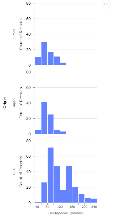
1-1. Row-Facet

origin (Europe, Japan, and USA) 毎の Horsepower の histogram を、各行 (row) に、表示します。

まずは facet operator を明記した書き方です。

Vl.new()
|> Vl.data_from_url("https://vega.github.io/vega-lite/data/cars.json")
|> Vl.facet(
  [row: [field: "Origin"]],
  Vl.new()
  |> Vl.mark(:bar)
  |> Vl.encode_field(:x, "Horsepower", type: :quantitative, bin: [maxbins: 15])
  |> Vl.encode(:y, aggregate: :count, type: :quantitative)
)

facet operator を明記せずに、row channel を指定すると Vega-Lite が自動的に上の facet operator の構文へコンバートしてくれます。ショートカットが可能です。

Vl.new()
|> Vl.data_from_url("https://vega.github.io/vega-lite/data/cars.json")
  |> Vl.mark(:bar)
  |> Vl.encode_field(:x, "Horsepower", type: :quantitative, bin: [maxbins: 15])
  |> Vl.encode(:y, aggregate: :count, type: :quantitative)
  |> Vl.encode_field(:row, "Origin")

どちらも下のグラフになります。

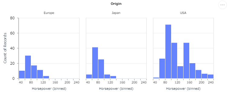
column channel を指定すると横並びになります。

Vl.new()
|> Vl.data_from_url("https://vega.github.io/vega-lite/data/cars.json")
  |> Vl.mark(:bar)
  |> Vl.encode_field(:x, "Horsepower", type: :quantitative, bin: [maxbins: 15])
  |> Vl.encode(:y, aggregate: :count, type: :quantitative)
  |> Vl.encode_field(:column, "Origin")

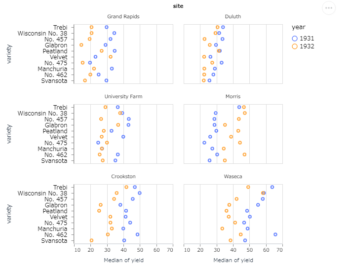
1-2. Wrapped Facet

facet channel を指定するやり方です。

Vl.new( name: "trellis_barley", height: [step: 12])
|> Vl.data_from_url("https://vega.github.io/vega-lite/data/barley.json")
|> Vl.mark(:point)
|> Vl.encode_field(:facet, "site", type: :ordinal, columns: 2,
                   sort: [op: "median", field: "yield"])
|> Vl.encode_field(:x, "yield", aggregate: :median, type: :quantitative,
                    scale: [zero: false])
|> Vl.encode_field(:y, "variety", type: :ordinal, sort: "-x")
|> Vl.encode_field(:color, "year", type: :nominal)

channel はザックリ言えば、座標のようなものと考えられます。例えば Data を 2次元座標 で表せば異なる point でも同じ座標にプロットしてしまうところを、3次元座標 で表せばキチンと異なる座標にプロットすることが可能なことがあります。当然 3次元の方がより多角的に Data を見ることができます。例えば (x, y) 座標の point に色を加え、つまりcolor軸 を設けて (x, y, color) 座標 で表現することが可能です。

2. layer

layer operator は一つのグラフを、他のグラフに重ね合わせるものです。
Layering views

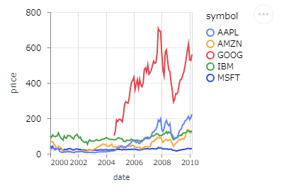
まず2つのグラフを示し、それらを layer operator で重ね合わせてみましょう。

株価の推移グラフです。

Vl.new()
|> Vl.data_from_url("https://vega.github.io/vega-lite/data/stocks.csv")
|> Vl.mark(:line)
|> Vl.encode_field(:x, "date", type: :temporal)
|> Vl.encode_field(:y, "price", type: :quantitative)
|> Vl.encode_field(:color, "symbol", type: :nominal)

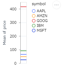
株価の平均のグラフです

Vl.new()
|> Vl.data_from_url("https://vega.github.io/vega-lite/data/stocks.csv")
|> Vl.mark(:rule)
|> Vl.encode_field(:y, "price", type: :quantitative, aggregate: :mean)
|> Vl.encode(:size, value: 2)
|> Vl.encode_field(:color, "symbol", type: :nominal)

rule mark はひとつの data point をひつつの line で表します。size で line の太さを指定します。

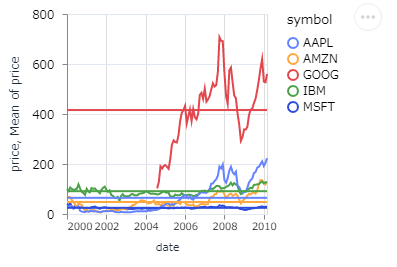
２つのグラフを layer operator で重ね合わせます。

Vl.new()
|> Vl.data_from_url("https://vega.github.io/vega-lite/data/stocks.csv")
|> Vl.layers([
  Vl.new()
  |> Vl.mark(:line)
  |> Vl.encode_field(:x, "date", type: :temporal)
  |> Vl.encode_field(:y, "price", type: :quantitative)
  |> Vl.encode_field(:color, "symbol", type: :nominal),   # カンマ注意
  Vl.new()
  |> Vl.mark(:rule)
  |> Vl.encode_field(:y, "price", type: :quantitative, aggregate: :mean)
  |> Vl.encode(:size, value: 2)
  |> Vl.encode_field(:color, "symbol", type: :nominal)
])

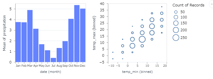
3. Concat

concat operator でグラフを合成することができます。

hconcat - 水平方向の合成
vconcat - 垂直方向の合成
concat - 一般的な合成 (wrappable)

Vl.new()
|> Vl.data_from_url("https://vega.github.io/vega-lite/data/weather.csv")
|> Vl.transform(filter: "datum.location === 'Seattle'")
|> Vl.concat(
  [
    Vl.new()
    |> Vl.mark(:bar)
    |> Vl.encode_field(:x, "date", time_unit: :month, type: :ordinal)
    |> Vl.encode_field(:y, "precipitation", aggregate: :mean),
    Vl.new()
    |> Vl.mark(:point)
    |> Vl.encode_field(:x, "temp_min", bin: true)
    |> Vl.encode_field(:y, "temp_max", bin: true)
    |> Vl.encode(:size, aggregate: :count)
  ],
  :horizontal
)

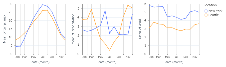
4. Repeat

repeat operator は field 配列 のそれぞれの要素に対して、グラフを作り出すためのショートカットです。Facet のように複数のプロットを生成しますが、Facet とは違って data set の完全な複製を許します。data の sub-set ではなく full-set です。

Vl.new()
|> Vl.data_from_url("https://vega.github.io/vega-lite/data/weather.csv")
|> Vl.repeat(
  ["temp_max", "precipitation", "wind"],
  Vl.new()
  |> Vl.mark(:line)
  |> Vl.encode_field(:x, "date", time_unit: :month)
  |> Vl.encode_repeat(:y, :repeat, aggregate: :mean)   # y channel = repeated field.
  |> Vl.encode_field(:color, "location")
)

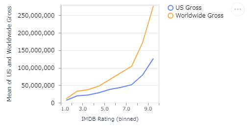
4-1. Multi-series Line Chart with Repeated Layers

repeat を layer と組み合わせて使い multi-series line chart を描くことができます。ここでは repeater field である data の値(datum)に color を map しています。

Vl.new()
|> Vl.data_from_url("https://vega.github.io/vega-lite/data/movies.json")
|> Vl.repeat(
  [layer: ["US Gross", "Worldwide Gross"]],
  Vl.new()
  |> Vl.mark(:line)
  |> Vl.encode_field(:x, "IMDB Rating", type: :quantitative, bin: true)
  |> Vl.encode_repeat(:y, :layer, aggregate: :mean, type: :quantitative,
                      title: "Mean of US and Worldwide Gross") 
  |> Vl.encode(:color, datum: [repeat: :layer], type: :nominal)

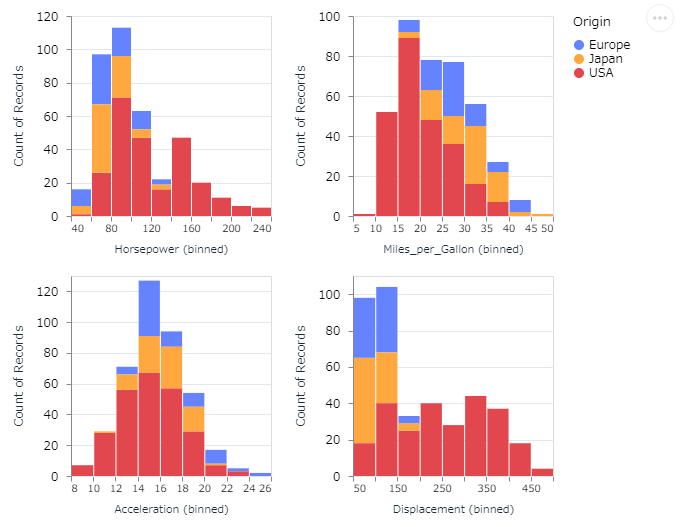
4-2. Repeated Histogram (Wrapped)

Vl.new(columns: 2)
|> Vl.repeat(
  ["Horsepower", "Miles_per_Gallon", "Acceleration", "Displacement"],
  Vl.new()
  |> Vl.data_from_url("https://vega.github.io/vega-lite/data/cars.json")
  |> Vl.mark(:bar)
  |> Vl.encode_repeat(:x, :repeat, bin: true)
  |> Vl.encode(:y, aggregate: :count)
  |> Vl.encode_field(:color, "Origin")
)

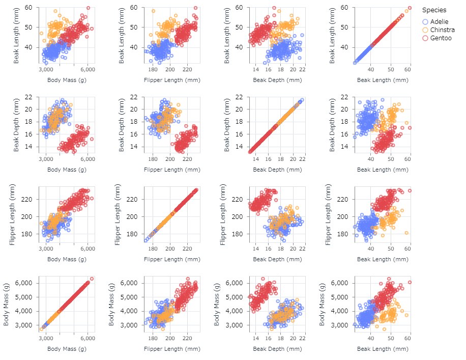
4-3. Scatterplot Matrix (SPLOM)

Vl.new()
|> Vl.data_from_url("https://vega.github.io/vega-lite/data/penguins.json")
|> Vl.repeat(
  [ row: ["Beak Length (mm)", "Beak Depth (mm)", "Flipper Length (mm)", "Body Mass (g)"],
  column: ["Body Mass (g)","Flipper Length (mm)","Beak Depth (mm)", "Beak Length (mm)"]],
  Vl.new(width: 110, height: 110)
  |> Vl.mark(:point)
  |> Vl.encode_repeat(:x, :column, type: :quantitative, scale: [zero: false])
  |> Vl.encode_repeat(:y, :row, type: :quantitative, scale: [zero: false])
  |> Vl.encode_field(:color, "Species", type: :nominal)
)

縦横のサイズを110にすることでギリギリ収まります。

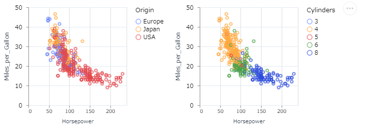
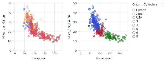
5. Resolution

Vega-Lite は scale domain (color domain など)が、結合されるべきかどうか決定します。もしそうなら、その軸と凡例はマージされます。そうでなければ、独立していなければなりません。Resolution によってこの決定を行います。

２つの repeated charts に対して、それぞれ2つの独立した color scales を与えます。この時 Vega-Lite は自動的に2つのchartに対して異なる凡例(Legend)を生成します。

Vl.new()
|> Vl.repeat(
  [column: ["Origin", "Cylinders"]],
  Vl.new()
  |> Vl.data_from_url("https://vega.github.io/vega-lite/data/cars.json")
  |> Vl.mark(:point)
  |> Vl.encode_field(:x, "Horsepower", type: :quantitative)
  |> Vl.encode_field(:y, "Miles_per_Gallon", type: :quantitative)
  |> Vl.encode_repeat(:color, :column, type: :nominal)
)
|> Vl.resolve(:scale, color: :independent)

最後の resolve 行を independent で追加することで、2つのグラフの凡例が独立して表示されます。

最後の resolve 行を消すと、凡例(Legend) が一つになってしまいます。

今回は以上です。

Vega-Lite の View Composition (Elixir, Livebook)