Stan, PyStanとは
Stanとは、C++をベースに実装された確率的プログラミング言語です。NUTSアルゴリズム (HMCを発展させたもの) を用いて、様々なベイズ推定を行うことができます。特徴として以下のようなものが挙げられます。
- 統計モデルの記述が簡単
- HMCなのでサンプリングが高速
- さまざまな確率分布を利用可能
PyStanはStanをPythonから扱うためのインターフェースを提供するパッケージです。Stanの文法に従ってモデルを記述し、コード実行時にモデルをコンパイルします。
PySTanのインストール
pipでインストール可能です。トレースプロットの描画のために arviz もインストールしておくと良いです。
$ pip install pystan
$ pip install arviz
PyStanによるベイズ推定
それでは実装していきます。まず必要なライブラリをインポートします。
import numpy as np
import pandas as pd
from scipy.stats import mstats

import matplotlib.pyplot as plt
import seaborn as sns
%matplotlib inline

import pystan
import arviz
1. 単回帰
ここではAuto MPGデータセットを使用します。UCI Machine Learning Repository からダウンロードできます。
データをpandas DataFrameに格納します。
column_names = ['MPG','Cylinders','Displacement','Horsepower','Weight',
                'Acceleration','Model Year','Origin']
df = pd.read_csv('auto-mpg.data', names=column_names, na_values = "?",
                 comment='\t', sep=" ", skipinitialspace=True)
燃費 (MPG : Mile per Gallon) は車両の重量 (Weight) に反比例するのではないか、という予想の下でこれを確かめてみます。
df['Weight_inv'] = df['Weight'].apply(lambda x: 1/x)
plt.scatter(df['Weight_inv'], df['MPG'])
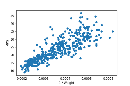
確かに重量の逆数は燃費と正の相関にありそうです。横軸の値によってばらつきが異なっているようですが、ここではひとまず以下のような統計モデルを仮定します。
$$MPG \sim Normal(a × Weight^{-1} +b, \sigma)$$
すなわち燃費は、重量の逆数の線形関数を平均とし、$\sigma$を分散とする正規分布に従うと仮定します。ここで出てきた$a, b, \sigma$が推定の対象となるパラメータになります。この統計モデルをStanの文法に従って記述すると以下のようになります。
stan_model = """
data {
    int N;
    real X[N];
    real Y[N];
}
parameters {
    real a;
    real b;
    real<lower=0> sigma;
}
model {
    for (n in 1:N) {
        Y[n] ~ normal(a * X[n] + b, sigma);
    }
}
"""
Stanのコードは以下のブロックが必要になります。
- data ... 観測データを記述
- parameters ... 推定対象のパラメータを記述
- model ... 仮定した統計モデルを記述
分散 sigma は非負の実数値をとるので、データ型を real<lower=0> とします。
モデルの記述が完了したら、これをコンパイルします。
sm = pystan.StanModel(model_code=stan_model)
観測データを辞書型で与え、MCMCサンプリングを行います。データ辞書のkeyは、Stanコードのdataブロックで定義した変数名に対応します。
pystan.StanModel.sampling の引数として、iter と warmup を与えています。iter はモンテカルロステップ数です。warmup ですが、定常状態に至るまでにしばらくかかるため、初期段階のサンプリングの結果は捨てた方が良いとされます。最初の何ステップを捨てるかを warmup で指定しています。
stan_data = {
    'N': df.shape[0],
    'X': df['Weight_inv'],
    'Y': df['MPG']
}
fit = sm.sampling(data=stan_data, iter=2000, warmup=500, chains=3, seed=123)
print(fit)
Inference for Stan model: anon_model_cdf2dd4817e02d2c4cf1f2106bb8e4c0.
3 chains, each with iter=2000; warmup=500; thin=1;
post-warmup draws per chain=1500, total post-warmup draws=4500.

        mean se_mean     sd   2.5%    25%    50%     75%  97.5%  n_eff   Rhat
a      6.6e4   54.18 2126.0  6.2e4  6.5e4  6.6e4   6.8e4  7.0e4   1540    1.0
b      -0.57    0.02   0.81  -2.12  -1.13  -0.56 -8.4e-3   1.01   1576    1.0
sigma   4.25  3.5e-3   0.16   3.94   4.14   4.24    4.35   4.56   1962    1.0
lp__  -772.7    0.03   1.24 -775.9 -773.3 -772.4  -771.8 -771.3   1571    1.0

Samples were drawn using NUTS at Sat Dec 19 07:48:35 2020.
For each parameter, n_eff is a crude measure of effective sample size,
and Rhat is the potential scale reduction factor on split chains (at
convergence, Rhat=1).
各推定値のRhatが1.0となっているため、定常状態に落ち着いていると解釈できます。
また、各推定値の平均値、50%信頼区間、95%信頼区間を確認できます。
各推定値のサンプリング結果は以下のようにアクセスできます。
fit.extract('a')['a']
# array([66799.22277616, 62788.84373091, 63577.82392938, ...,
#        63620.47069878, 63571.6229788 , 67382.64630103])
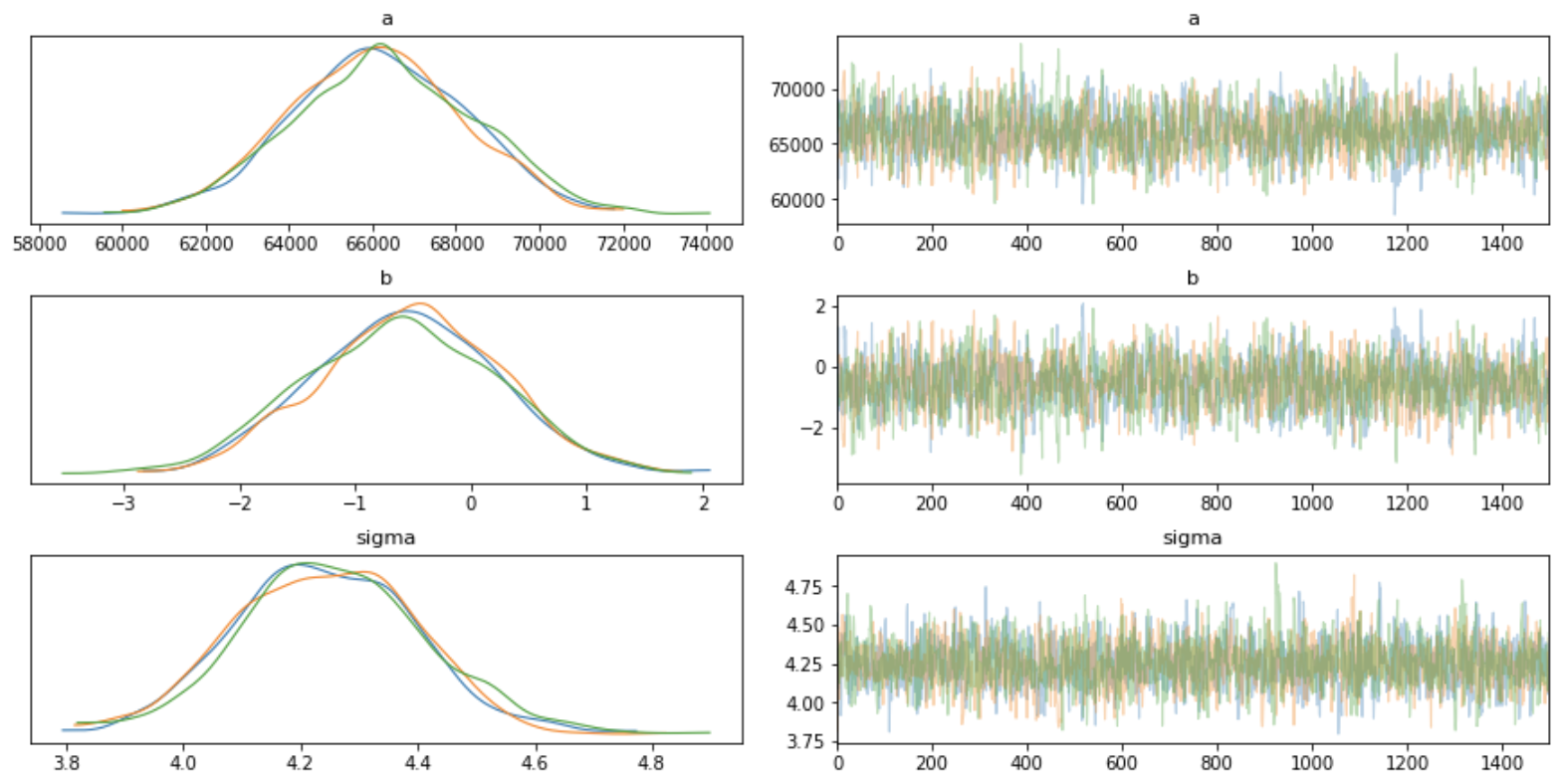
サンプリング結果の分布とトレースプロットを次のように表示できます。
fig = arviz.plot_trace(fit)
それではa, bの推定値を用いて予測直線を信頼区間とともに描いてみましょう。
a, b = 6.6e4, -0.57
x = np.linspace(0.0002, 0.0006, 100)
y = a * x + b
plt.plot(x, y, color='red')
plt.scatter(df['Weight_inv'], df['MPG'])
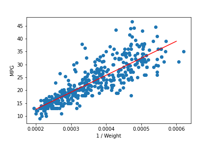
概ね良い推定が出来ていることが確認できます。
2. ロジスティック回帰
続いてロジスティック回帰です。今度は予測回帰曲線を信頼区間とともに表示してみましょう。
scikit-learnの乳がんデータセット (breast_cancer) を使用します。細胞の半径 (mean radius) を説明変数、悪性かどうか (malignant) を目的変数とします。
from sklearn.datasets import load_breast_cancer

bc = load_breast_cancer()
df = pd.DataFrame(bc.data, columns=bc.feature_names)
df['benign'] = bc.target
df['malignant'] = df['benign'].apply(lambda x: 1 if x == 0 else 0)
散布図を確認します。
plt.scatter(df['mean radius'], df['malignant'])
plt.xlabel('Mean radius')
plt.ylabel('Malignant')
plt.xlim([5, 30])
plt.yticks([0, 1])

細胞の半径 (mean radius) が大きいほど、悪性である確率が大きい傾向が読み取れます。以下のようなロジスティック回帰モデルを仮定します。
$$Malignant \sim \exp(a \times MeanRadius + b))$$
単回帰同様、Stanコードを記述し、コンパイルします。
モデルの記述において、ロジスティック回帰では bernoulli_logit を使用します。
stan_model = """
data {
    int N;
    real X[N];
    int<lower=0, upper=1> Y[N];
}
parameters {
    real a;
    real b;
}
model {
    for (n in 1:N) {
        Y[n] ~ bernoulli_logit(a*X[n] + b);
    }
}
"""
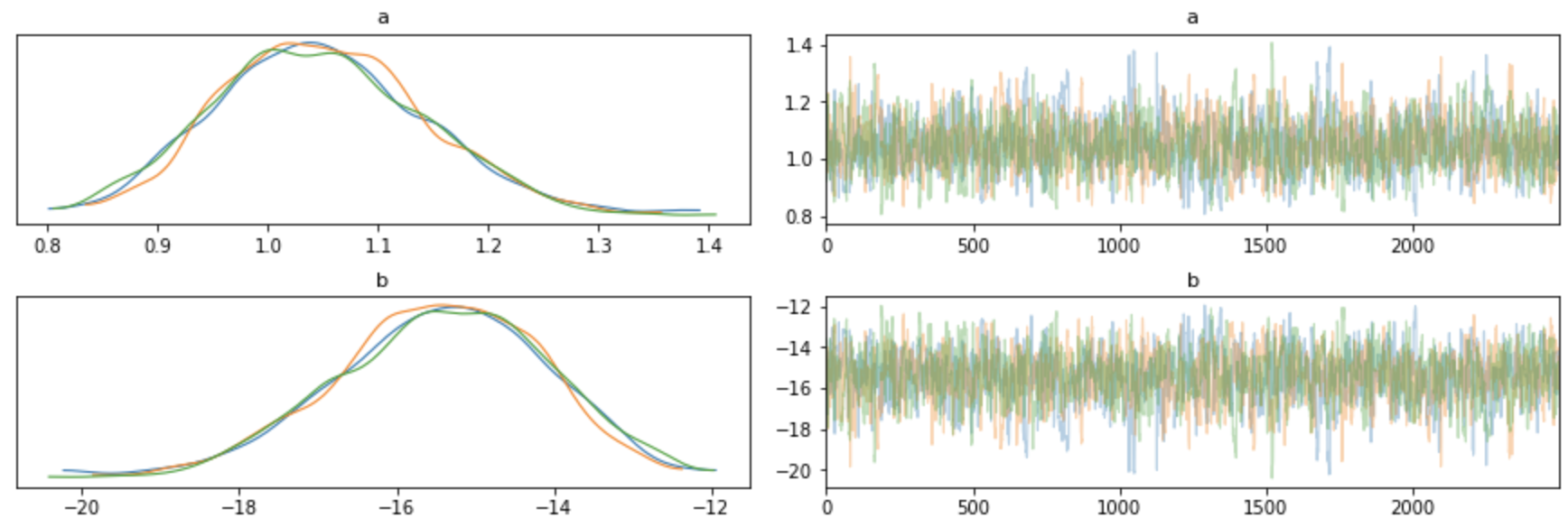
観測データを与え、MCMCサンプリングを行います。
また、トレースプロットとともに出力結果を表示します。
stan_data = {
    'N': df.shape[0],
    'X': df['mean radius'],
    'Y': df['malignant']
}
fit = sm.sampling(data=stan_data, iter=3000, warmup=500, chains=3, seed=123)
print(fit)

fig = arviz.plot_trace(fit)
Inference for Stan model: anon_model_961ca63f5fca60aa2e92ea6e3198f2fb.
3 chains, each with iter=3000; warmup=500; thin=1;
post-warmup draws per chain=2500, total post-warmup draws=7500.

       mean se_mean     sd   2.5%    25%    50%    75%  97.5%  n_eff   Rhat
a      1.05  2.8e-3   0.09   0.88   0.98   1.04   1.11   1.24   1166    1.0
b    -15.46    0.04   1.35 -18.23 -16.32 -15.41  -14.5 -13.02   1160    1.0
lp__ -166.0    0.02   0.98 -168.6 -166.4 -165.7 -165.2 -165.0   1896    1.0

Samples were drawn using NUTS at Sat Dec 19 13:40:51 2020.
For each parameter, n_eff is a crude measure of effective sample size,
and Rhat is the potential scale reduction factor on split chains (at
convergence, Rhat=1).
RHat=1.0ということで、よく収束していることが分かります。
a, bの推定値は回帰曲線の表示に利用するので変数に格納しておきます。
a, b = 1.05, -15.46
続いて、サンプリング結果を用いて信頼区間を求めていきます。
前述の通り、extract() メソッドでサンプリング結果を抽出します。予測区間を [0, 30] としてサンプリング回数 (2500×3=7500回) 分のロジスティック回帰曲線を求め、pandas DataFrameに格納します。計算結果をもとに、scipy.stats.mstats.mquantiles を用いて50%信頼区間、99%信頼区間を求めます。
ms_a = fit.extract('a')['a']
ms_b = fit.extract('b')['b']

x = np.linspace(0, 30, 100)
logistic_func = lambda x: 1.0 / (1.0+np.exp(-x))
df_lines = pd.DataFrame([])
for i in range(x.shape[0]):
    df_lines[i] = logistic_func(ms_a*x[i] + ms_b)

low_y50, high_y50 = mstats.mquantiles(df_lines, [0.25, 0.75], axis=0)
low_y99, high_y99 = mstats.mquantiles(df_lines, [0.005, 0.995], axis=0)
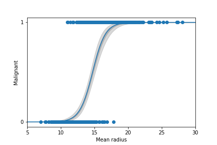
それでは信頼区間とともに、観測データおよび回帰曲線を描画してみましょう。
plt.fill_between(x, low_y50, high_y50, alpha=0.6, color='darkgray')
plt.fill_between(x, low_y99, high_y99, alpha=0.3, color='gray')
plt.plot(x, logistic_func(a*x+b))
plt.scatter(df['mean radius'], df['malignant'])
plt.xlabel('Mean radius')
plt.ylabel('Malignant')
plt.xlim([5, 30])
plt.yticks([0, 1])
まとめ
以上、PyStanの紹介とPyStanによる単回帰とロジスティック回帰の実装でした!
良いデータセットが見つかれば階層ベイズなんかも記事に出来たらと思います。