はじめに
- PyCaretは僅かなコーディングで機械学習ができるライブラリです。
- 非常に便利なライブラリですが、TensorFlowやPyTorchのようなニューラルネットワークモデルには対応していません(scikit-learnのMLPは実装可能)。
- 本稿ではPycaretを前処理用ツールとして使い、ニューラルネットワークモデル(TabNet)を構築する手法を紹介します。
前処理の自動化
PyCaretの基本的な使い方は割愛します。
初めて使う方は以下の記事を参照ください。
※環境はgoogle colaboratoryで実行しています。
今回はボストン不動産価格データを使います。
   from pycaret.datasets import get_data
   from pycaret.regression import *
   dataset = get_data('boston')
setup関数を使って前処理を行います。
   exp = setup(dataset,
               session_id=123, #ランダムシードの値
               train_size = 0.7, #学習データとテストデータを7:3に分割
               target = 'medv', #目的関数
               categorical_features = ['chas'], #カテゴリー変数
               numeric_features = ['rad'], #数値変数
               normalize = True, #標準化の有無
               normalize_method = 'zscore', #標準化の方法
               )
前処理の詳細は下図になります。

前処理されたデータを確認します。get_configで全ての説明変数のデータを取得します。
   X = get_config('X') #全ての説明変数
   X
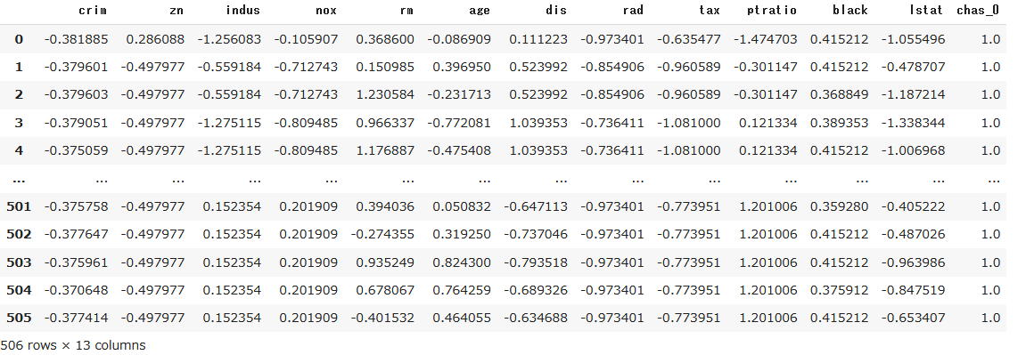
numeric_features(chas以外)は標準化され、
categorical_featuresであるchasはダミー変数になりました(元からダミー変数でしたが)。
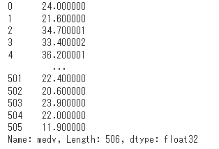
続いて目的変数medvを確認します。
   y = get_config('y') # 全ての目的変数
   y
ここでは使用しませんが、分割された学習データ、テストデータの確認も可能です。上記の「Transformed Train Set」、「Transformed Test Set」にあたります。
   X_train = get_config('X_train') # 分割後の学習用説明変数
   X_train.head()
目的変数は以下です。
   y_train = get_config('y_train') # 分割後の学習用目的変数
   y_train.head()
同様に分割されたテストデータ「Transformed Test Set」は以下です。
   X_test = get_config('X_test') # 分割後のテスト用説明変数
   X_test.head()
目的変数は以下です。
   y_test = get_config('y_test') # 分割後のテスト用目的変数
   y_test.head()
前処理した学習データとテストデータを結合して前処理後のデータセットを作成します。
   df=pd.merge(X, y,left_index=True,right_index=True)
   df
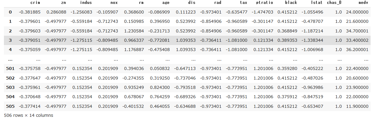
実は本稿で重要なのはここまでです。
前処理されたデータにさらにひと手間加えるも良し、好きなモデルに組み込むも良しです。
PyCaretをデータ前処理ツールとして使ってみたら如何でしょうかという提案でした。
3. TabNetの構築
以降はほぼ蛇足になりますがTabNetでの学習です。
   #ライブラリ
   import torch
   from torch import nn
   import torch.optim as optim
   import torch.nn.functional as F
   from torch.optim.lr_scheduler import ReduceLROnPlateau
   from sklearn.model_selection import StratifiedKFold
   from pytorch_tabnet.tab_model import TabNetRegressor
   import os
   import random
   import pandas as pd
   import numpy as np
   import seaborn as sns
   import matplotlib.pyplot as plt
   from sklearn.model_selection import train_test_split
   from sklearn.metrics import r2_score
   from sklearn.metrics import mean_absolute_error
   from sklearn.metrics import mean_squared_error

   %matplotlib inline

   def seed_everything(seed_value):
       random.seed(seed_value)
       np.random.seed(seed_value)
       torch.manual_seed(seed_value)
       os.environ["PYTHONHASHSEED"] = str(seed_value)

       if torch.cuda.is_available():
           torch.cuda.manual_seed(seed_value)
           torch.cuda.manual_seed_all(seed_value)
           torch.backends.cudnn.deterministic = True
           torch.backends.cudnn.benchmark = False

   seed_everything(10)

   # ランダムシード値
   RANDOM_STATE = 10

   # 学習データと評価データの割合
   TEST_SIZE = 0.3

   # 学習データと評価データを作成
   x_train, x_test, y_train, y_test = train_test_split(
       df.iloc[:, 0 : df.shape[1] - 1],
       df.iloc[:, df.shape[1] - 1],
       test_size=TEST_SIZE,
       random_state=RANDOM_STATE,
   )

   # trainのデータセットの3割をモデル学習時のバリデーションデータとして利用する
   x_train, x_valid, y_train, y_valid = train_test_split(
       x_train, y_train, test_size=TEST_SIZE, random_state=RANDOM_STATE
   )
   # モデルのパラメータ
   tabnet_params = dict(
       n_d=8,
       n_a=8,
       n_steps=8,
       gamma=0.2,
       seed=10,
       lambda_sparse=1e-3,
       optimizer_fn=torch.optim.Adam,
       optimizer_params=dict(lr=2e-2, weight_decay=1e-5),
       mask_type="entmax",
       scheduler_params=dict(
           max_lr=0.01,
           steps_per_epoch=int(x_train.shape[0] / 256),
           epochs=200,
           is_batch_level=True,
       ),
       verbose=5,
   )

   # model
   model = TabNetRegressor(**tabnet_params)

   model.fit(
       X_train=x_train.values,
       y_train=y_train.values.reshape(-1, 1),
       eval_set=[(x_valid.values, y_valid.values.reshape(-1, 1))],
       eval_metric=["rmse"],
       max_epochs=200,
       patience=30,
       batch_size=256,
       virtual_batch_size=128,
       num_workers=2,
       drop_last=False,
       loss_fn=torch.nn.functional.l1_loss,
   )
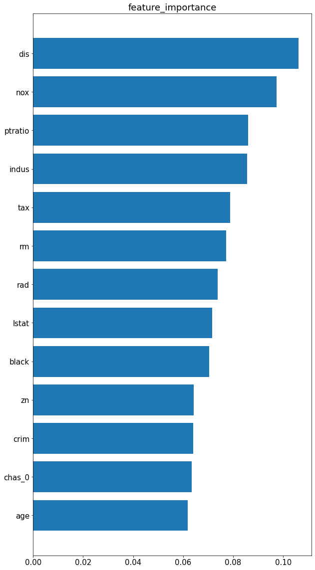
特徴量の重要度を表示します。
   # Feature Importance

   feat_imp = pd.DataFrame(model.feature_importances_, index=X.columns)
   feature_importance = feat_imp.copy()

   feature_importance["imp_mean"] = feature_importance.mean(axis=1)
   feature_importance = feature_importance.sort_values("imp_mean")
   plt.figure(figsize=(10,20))
   plt.tick_params(labelsize=15)
   plt.barh(feature_importance.index.values, feature_importance["imp_mean"])
   plt.title("feature_importance", fontsize=18)
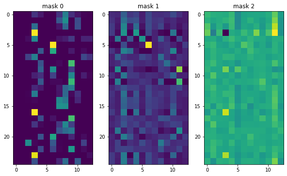
各特徴のマスクを表示します。
   # Mask(Local interpretability)
   explain_matrix, masks = model.explain(x_test.values)

   fig, axs = plt.subplots(1, 3, figsize=(10, 7))

   for i in range(3):
       axs[i].imshow(masks[i][:25])
       axs[i].set_title(f"mask {i}")
評価指標を算出します。あまり結果は良くないです。
   # TabNet推論
   y_pred = model.predict(x_test.values)

   # 評価
   def calculate_scores(true, pred):
       scores = {}
       scores = pd.DataFrame(
           {
               "R2": r2_score(true, pred),
               "MAE": mean_absolute_error(true, pred),
               "MSE": mean_squared_error(true, pred),
               "RMSE": np.sqrt(mean_squared_error(true, pred)),
           },
           index=["scores"],
       )
       return scores


   scores = calculate_scores(y_test, y_pred)
   print(scores)

テストデータで推論する方法
テストデータを使って推論をする場合は以下のようにします。
ここで重要なのはsetup関数の設定を学習データと揃える事です。
   test = pd.read_csv("test.csv")
   exp2 = setup(test,
               session_id=123, #ランダムシードの値
               #train_sizeは無くてOK
               target = 'medv', #目的関数
               categorical_features = ['chas'], #カテゴリー変数
               numeric_features = ['rad'], #数値変数
               normalize = True, #標準化の有無
               normalize_method = 'zscore', #標準化の方法
               )
テストデータの前処理が終わったら全ての説明変数だけを取り出して推論に回します。
   # 全説明変数
   X = get_config('X')

   # TabNet推論
   y_pred = model.predict(X.values)
   y_pred=pd.DataFrame(y_pred)
さいごに
如何だったでしょうか?
以下の記事では「PyCaretはscikit-learnモデル以外も対応できるよ!」とありますが、
ニューラルネットワークへの適応は出来なさそうなので今回の手法は有効ではと思います。
参考
https://qiita.com/maskot1977/items/5de6605806f8918d2283
https://pycaret.org/preprocessing/