今回の話
前回は、Sonnetの基本的な使い方について説明しました。今回は応用として、Xceptionモデルの実装と学習を行ってみます。
本当はSonnetを使った場合と直にTensorFlowでコードを書いた場合でどれくらい可読性が上がるか、とかいろいろやりたかったのですが、体調をぶっ壊してしまったので間に合わず。。。orz
Xceptionモデルそのものの解説は今回は他に任せるとして、Sonnetを利用してどのように実装できるか、ということを中心に解説していきます。なぜXceptionモデルを選んだかというと、モデルの中に同じ箇所の繰り返しが出てきたり、構造が同じでパラメータが違う箇所が複数出てきたりと、モジュール化することですっきりコーディングできそうな感じがしたからです。まぁGoogLeNetのようなInceptionモデルでもよかったのですが、新しいもの好きなので。。
追記@2017/12/18
今回実装したコードはGithubにあります。
Xception
Xceptionモデルは、2017年4月にFrançois Chollet氏によって発表されたモデルで、Inceptionモデルからパラメータ削減を目指す方向で改良を行ったものです。詳しい内容はここでは省略します。ちなみにChollet氏はKerasの作者でもあります。
Xceptionモデルの構造は以下のようになっています。
 ('Xception: Deep Learning with Depthwise Separable Convolutions'より引用)
大きく分けて3つのパーツからなり、どのflowでもskip connectionが存在します。
Entry flow
Entry flowでは最初にconvolutionとReLUを2回繰り返したあと、skip connection + separable convolutionのセットを3回繰り返します。このseparable convolutionが、パラメータ削減の大きなポイントとなるみたいです。この部分を繰り返しコーディングするのは大変なので、Sonnetのモジュールを作って簡略化してしまいます。
# entry flow module
class EntryFlowModule(snt.AbstractModule):
    def __init__(self, output_channels, num, name='EntryFlowModule'):
        self.output_channels = output_channels
        self.num = str(num)

        super(EntryFlowModule, self).__init__(name=name)

        with self._enter_variable_scope():
            self.resconv_e1 = snt.Conv2D(output_channels=self.output_channels, kernel_shape=1, stride=2, name='resconv_e{}'.format(self.num))
            self.bn_rese1 = snt.BatchNorm(name='bn_rese{}'.format(self.num))

            self.sepconv_e1 = snt.SeparableConv2D(output_channels=self.output_channels, channel_multiplier=1, kernel_shape=3, name='sepconv_e{}1'.format(self.num))
            self.bn_sepe1 = snt.BatchNorm(name='bn_sepe{}1'.format(self.num))

            self.sepconv_e2 = snt.SeparableConv2D(output_channels=self.output_channels, channel_multiplier=1, kernel_shape=3, name='sepconv_e{}2'.format(self.num))
            self.bn_sepe2 = snt.BatchNorm(name='bn_sepe{}2'.format(self.num))

    def _build(self, x, is_train):
        residual = self.resconv_e1(x)
        residual = self.bn_rese1(residual, is_train)

        h = self.sepconv_e1(x)
        h = self.bn_sepe1(h, is_train)

        h = self.sepconv_e2(tf.nn.relu(h, name='relu_e{}'.format(self.num)))
        h = self.bn_sepe2(h, is_train)

        h = tf.nn.max_pool(h, ksize=[1, 3, 3, 1], strides=[1, 2, 2, 1], padding='SAME', name='maxpool_e{}'.format(self.num))
        h = tf.add(h, residual, name='add_e{}'.format(self.num))

        return h
skip connection + separable convolutionの部分です。書き方は前回に説明した通りですね。
separable convolutionはSonnetのモジュールでSeparableConv2Dが用意されているので、こちらを使います。この部分は箇所によって出力チャネル数が違うので、コンストラクタでoutput_channelsを指定します。
Middle flow
Middle flowでは、skip connection + separable convolutionのセットを8回繰り返します。もちろん全部書くのは大変なのでモジュール化して使いまわします。
# middle flow module
class MiddleFlowModule(snt.AbstractModule):
    def __init__(self, num, name='MiddleFlowModule'):
        self.num = str(num)
        super(MiddleFlowModule, self).__init__(name=name)

        with self._enter_variable_scope():
            self.sepconv_m1 = snt.SeparableConv2D(output_channels=728, channel_multiplier=1, kernel_shape=3, name='sepconv_m{}1'.format(self.num))
            self.bn_sepm1 = snt.BatchNorm(name='bn_sepm{}1'.format(self.num))

            self.sepconv_m2 = snt.SeparableConv2D(output_channels=728, channel_multiplier=1, kernel_shape=3, name='sepconv_m{}2'.format(self.num))
            self.bn_sepm2 = snt.BatchNorm(name='bn_sepm{}2'.format(self.num))

            self.sepconv_m3 = snt.SeparableConv2D(output_channels=728, channel_multiplier=1, kernel_shape=3, name='sepconv_m{}3'.format(self.num))
            self.bn_sepm3 = snt.BatchNorm(name='bn_sepm{}3'.format(self.num))

    def _build(self, x, is_train):
        res = x
        h = self.sepconv_m1(tf.nn.relu(x, name='relu_m{}1'.format(self.num)))
        h = self.bn_sepm1(h, is_train)

        h = self.sepconv_m2(tf.nn.relu(h, name='relu_m{}2'.format(self.num)))
        h = self.bn_sepm2(h, is_train)

        h = self.sepconv_m3(tf.nn.relu(h, name='relu_m{}3'.format(self.num)))
        h = self.bn_sepm3(h, is_train)

        h = tf.add(h, res, name='add_m{}'.format(self.num))

        return h
Middle flowはどの部分もパラメータが同じなので、全く同じモジュールを繰り返し使います。
Exit flow
Exit flowでは繰り返しの箇所は登場しませんが、地味にseparable convolutionが多いのと層数が多いので、モジュールで一つにまとめてしまいます。
# exit flow module
class ExitFlowModule(snt.AbstractModule):
    def __init__(self, name='ExitFlowModule'):
        super(ExitFlowModule, self).__init__(name=name)

        with self._enter_variable_scope():
            self.resconv_ex1 = snt.Conv2D(output_channels=1024, kernel_shape=1, stride=2, name='resconv_ex1')
            self.bn_resex1 = snt.BatchNorm(name='bn_resex1')

            self.sepconv_ex1 = snt.SeparableConv2D(output_channels=728, channel_multiplier=1, kernel_shape=3, name='sepconv_ex1')
            self.bn_sepex1 = snt.BatchNorm(name='bn_sepex1')

            self.sepconv_ex2 = snt.SeparableConv2D(output_channels=1024, channel_multiplier=1, kernel_shape=3, name='sepconv_ex2')
            self.bn_sepex2 = snt.BatchNorm(name='bn_sepex2')

            self.sepconv_ex3 = snt.SeparableConv2D(output_channels=1536, channel_multiplier=1, kernel_shape=3, name='sepconv_ex3')
            self.bn_sepex3 = snt.BatchNorm(name='bn_sepex3')

            self.sepconv_ex4 = snt.SeparableConv2D(output_channels=2048, channel_multiplier=1, kernel_shape=3, name='sepconv_ex4')
            self.bn_sepex4 = snt.BatchNorm(name='bn_sepex4')

    def _build(self, x, is_train):
        residual = self.resconv_ex1(x)
        residual = self.bn_resex1(residual, is_train)

        h = self.sepconv_ex1(tf.nn.relu(x, name='relu_ex1'))
        h = self.bn_sepex1(h, is_train)

        h = self.sepconv_ex2(tf.nn.relu(h, name='relu_ex2'))
        h = self.bn_sepex2(h, is_train)

        h = tf.nn.max_pool(h, ksize=[1, 3, 3, 1], strides=[1, 2, 2, 1], padding='SAME', name='maxpool_ex')
        h = tf.add(h, residual, name='add_ex2')

        h = self.sepconv_ex3(h)
        h = tf.nn.relu(self.bn_sepex3(h, is_train), name='relu_ex3')

        h = self.sepconv_ex4(h)
        h = tf.nn.relu(self.bn_sepex4(h, is_train), name='relu_ex4')

        # in paper, kernel size of global pooling is 10.
        # in this code, kernel size is 5 cause length of input image is 149.
        h = tf.nn.avg_pool(h, ksize=[1, 5, 5, 1], strides=[1, 1, 1, 1], padding='VALID', name='global_avg_pool')
        h = snt.BatchFlatten(name='flatten')(h)

        return h
ここで、本当は論文通りのパラメータで実験したかったのですが、GPUメモリが足りなかったので入力画像のサイズを299×299から149×149に下げています。そのため、最後のglobal average poolingのカーネルサイズを10から5に変更してあります。
モデル全体
モデル全体は、作成したモジュールを使うと次のようになります。
# Xception module
class Xception(snt.AbstractModule):
    def __init__(self, output_size, name='Xception'):

        self.output_size = output_size

        super(Xception, self).__init__(name=name)
        # input size = (149, 149)
        with self._enter_variable_scope():
            # Entry Flow
            self.conv_e1 = snt.Conv2D(output_channels=32, kernel_shape=3, stride=2, name='conv_e1')
            self.bn_e1 = snt.BatchNorm(name='bn_e1')
            self.conv_e2 = snt.Conv2D(output_channels=64, kernel_shape=3, name='conv_e2')
            self.bn_e2 = snt.BatchNorm(name='bn_e2')

            self.entry_flow_1 = EntryFlowModule(output_channels=128, num=1, name='entry_flow_1')
            self.entry_flow_2 = EntryFlowModule(output_channels=256, num=2, name='entry_flow_2')
            self.entry_flow_3 = EntryFlowModule(output_channels=728, num=3, name='entry_flow_3')

            # Middle Flow
            self.middles = [MiddleFlowModule(num=n, name='middle_flow_{}'.format(str(n))) for n in range(1, 9)]

            # Exit Flow
            self.exit_flow = ExitFlowModule(name='exit_flow')

            self.l1 = snt.Linear(output_size=256, name='l1')
            self.l2 = snt.Linear(output_size=self.output_size, name='l2')

    def _build(self, inputs, is_train, dropout_rate=0.5):
        # input size = (149, 149)
        # in paper, input image size = (299, 299)

        # Entry Flow
        h = self.conv_e1(inputs)
        h = tf.nn.relu(self.bn_e1(h, is_train), name='relu_1')
        h = self.conv_e2(h)
        h = tf.nn.relu(self.bn_e2(h, is_train), name='relu_2')

        h = self.entry_flow_1(h, is_train)
        h = self.entry_flow_2(h, is_train)
        h = self.entry_flow_3(h, is_train)

        # Middle Flow
        for mm in self.middles:
            h = mm(h, is_train)

        # Exit Flow
        h = self.exit_flow(h, is_train)

        h = tf.nn.relu(self.l1(h), name='relu_l1')
        feature = h
        h = tf.nn.dropout(h, keep_prob=dropout_rate if is_train else 1., name='dropout')
        y = self.l2(h)

        return y, feature
作ったモジュールを使いまわすことですっきり書くことができます。最後の全結合層は2層とし、1層目の出力次元数は256固定としました。
データセット
学習するデータセットは17 Category Flower Datasetを使いました。なぜかというと、お花に癒されたかったからです。。。

きれいだなぁ
このような花の画像を17カテゴリに分類する問題です。
前回と同じように、データ供給部分もモジュールで作ります。
データをダウンロードすると、画像ファイル名はimage_1037.jpgみたいな感じで付いています。数字部分の1桁目がクラスタラベルとなるので、画像ファイルを読み込んでファイル名からラベルを抽出します。
# coding: utf-8
import tensorflow as tf
import sonnet as snt
import numpy as np
from PIL import Image


def _one_hot(length, value):
    tmp = np.zeros(length, dtype=np.float32)
    tmp[value] = 1.
    return tmp


class FlowerDataSet(snt.AbstractModule):
    def __init__(self, file_list, image_size, batch, name='FlowerDataSet'):
        super(FlowerDataSet, self).__init__(name=name)
        self.filelist = file_list

        imgs = []
        lbls = []
        self.image_size = image_size
        for f in self.filelist:
            img = Image.open(f)
            img = img.resize(self.image_size)
            imgs.append(np.asarray(img))
            lbls.append(_one_hot(17, (int(f.split('_')[-1][:-4]) - 1) // 80))
        imgs = np.asarray(imgs)
        lbls = np.asarray(lbls)

        self.num_data = len(self.filelist)
        self.images = tf.constant(imgs)
        self.labels = tf.constant(lbls, dtype=tf.float32)

        self.batch = batch

    def _build(self, is_train):
        if is_train:
            indices = tf.random_uniform([self.batch], 0, self.num_data, tf.int64)
            x_ = tf.cast(tf.gather(self.images, indices), tf.float32)

            # data augmentation
            # flip left-right
            x_tmp = tf.split(x_, self.batch, axis=0)
            flipped = []
            for x_t in x_tmp:
                flipped.append(tf.image.random_flip_left_right(tf.squeeze(x_t)))
            distorted_x = tf.stack(flipped, axis=0)

            # brightness
            distorted_x = tf.image.random_brightness(distorted_x, max_delta=63)

            # contrast
            x = tf.image.random_contrast(distorted_x, lower=0.2, upper=1.8)

            y_ = tf.gather(self.labels, indices)

            return x, y_
        else:
            return tf.cast(self.images, tf.float32), self.labels

    @staticmethod
    def cost(logits, target):
        return tf.losses.softmax_cross_entropy(logits=logits, onehot_labels=target)

    @staticmethod
    def evaluation(logits, target):
        correct_prediction = tf.equal(tf.argmax(logits, 1, name='argmax_y'), tf.argmax(target, 1, name='argmax_t'))
        return tf.reduce_mean(tf.cast(correct_prediction, tf.float32))
コンストラクタで画像ファイルがあるディレクトリを指定して画像をインポートし、リサイズしておきます。
_build()は、学習時と評価時で異なる挙動をします。学習時は学習用データからランダムにバッチサイズ分選択し、data augmentationを行った上でラベルと一緒に返します。一方で評価は評価用データをラベルと一緒にそのまま返します。
data augmentationでは
- 左右反転
- 輝度変更
- コントラスト変更
をランダムに行っています。
学習
これでモデル構築とデータの用意ができたので、いよいよ学習です。
基本的な流れは前回と同じです。今回は前回行わなかったWeight Decayと、学習率の減衰スケジューリングを入れて学習してみます。本当は入れる前/入れた後で比較しなきゃいけないのだが、時間がな(ry
計算グラフを構築するところまでのコードはこのようになります。
# パラメータをセット
FLAGS = tf.flags.FLAGS
tf.flags.DEFINE_integer("num_training_iterations", 2000, "Number of iterations to train for.")
tf.flags.DEFINE_integer("report_interval", 100, "Iterations between reports (samples, valid loss).")
tf.flags.DEFINE_integer("batch_size", 100, "Batch size for training.")
tf.flags.DEFINE_integer("output_size", 17, "Size of output layer.")
tf.flags.DEFINE_float("weight_decay_rate", 1.e-4, "Rate for Weight Decay.")
tf.flags.DEFINE_float("train_ratio", 0.8, "Ratio of train data in the all data.")
tf.flags.DEFINE_float("init_lr", 1.e-3, "Initial learning rate.")
tf.flags.DEFINE_integer("decay_interval", 500, "lr decay interval.")
tf.flags.DEFINE_float("decay_rate", 0.5, "lr decay rate.")

# Xceptionモジュール
xception = Xception(FLAGS.output_size, name='Xception')

image_dir_path = 'jpg'
filelist = list(filter(lambda z: z[-4:] == '.jpg', os.listdir(image_dir_path)))
filelist = np.asarray([os.path.join(image_dir_path, f) for f in filelist])
idx = np.arange(len(filelist))
np.random.shuffle(idx)
border = int(len(filelist) * FLAGS.train_ratio)

# Flower data set モジュール
dataset_train = FlowerDataSet(file_list=filelist[:border], image_size=(149, 149), batch=FLAGS.batch_size, name='Flower_dataset_train')
dataset_test = FlowerDataSet(file_list=filelist[border:], image_size=(149, 149), batch=FLAGS.batch_size, name='Flower_dataset_test')

# 計算グラフ
# train
train_x, train_y_ = dataset_train(is_train=True)
train_y, _ = xception(train_x, is_train=True)
ce_loss = dataset_train.cost(logits=train_y, target=train_y_)
# L2正則化
reg_loss = tf.get_collection(tf.GraphKeys.REGULARIZATION_LOSSES)
# total loss (with Weight Decay)
loss = tf.add(ce_loss, FLAGS.weight_decay_rate * tf.reduce_sum(reg_loss), name='total_loss')
tf.summary.scalar('loss', loss)
tf.summary.image('train_batch', train_x)

# test
test_x, test_y_ = dataset_test(is_train=False)
test_y, feature = xception(test_x, is_train=False)
accuracy = dataset_test.evaluation(logits=test_y, target=test_y_)
tf.summary.scalar('accuracy', accuracy)

# optimizer
global_step = tf.Variable(0, trainable=False, name='global_step')
learning_rate = tf.train.exponential_decay(FLAGS.init_lr, global_step, FLAGS.decay_interval, FLAGS.decay_rate,
                                           staircase=True, name='learning_rate')
train_step = tf.train.AdamOptimizer(learning_rate).minimize(loss, global_step=global_step)
tf.summary.scalar('lr', learning_rate)
パラメータを用意→モジュールをセット→計算グラフを構築 という流れは前回と同じですね。一応前回に合わせて、学習用と評価用のデータ供給モジュールを分けて作成しています。そのため、データセットを分割してからそれぞれのモジュールに画像ファイルリストを分配しています。データ供給モジュールを1つにまとめて、コンストラクタでデータを分割して保持しておき、_build()で出し分けても良いかもしれません。
lossを計算している部分は以下の箇所です。
ce_loss = dataset_train.cost(logits=train_y, target=train_y_)
# L2正則化
reg_loss = tf.get_collection(tf.GraphKeys.REGULARIZATION_LOSSES)
# total loss (with Weight Decay)
loss = tf.add(ce_loss, FLAGS.weight_decay_rate * tf.reduce_sum(reg_loss), name='total_loss')
ce_lossはデータセットモジュールに定義したsoft-max cross entropyですね。Weight Decayを入れるには、パラメータの正則化lossを集めてきて足し込む必要があります。モデル全体のlossはどうやら一箇所にまとめて保存されているらしく、それを呼び出す関数がtf.get_collection()です。そのうち、正則化lossのみ取り出すには引数にtf.GraphKeys.REGULARIZATION_LOSSESを指定すれば良いみたいです。各層のパラメータの正則化lossがタプルで返ってくるので、tf.reduce_sum()で和をとってdecay rateを乗じてもとのce_lossに足せばWeight Decayを実現できます。(記事を執筆している日にインターンの学生にこれを教えてもらいました。。。ありがとう!)
optimizerの設定部分は以下の箇所です。
global_step = tf.Variable(0, trainable=False, name='global_step')
learning_rate = tf.train.exponential_decay(FLAGS.init_lr, global_step, FLAGS.decay_interval, FLAGS.decay_rate,
                                           staircase=True, name='learning_rate')
train_step = tf.train.AdamOptimizer(learning_rate).minimize(loss, global_step=global_step)
通常はtrain_step = tf.train.AdamOptimizer(1.e-4).minimize(loss)みたいな感じでoptimizerをセットすれば良いのですが、あるステップで学習率を変更(減衰のみ)したい場合は、学習ステップ数と学習率の変数を別途作成してその変数間でスケジューリングを設定してやる必要があります。
学習ステップはglobal_stepとして、初期値0の学習対象でない変数を定義します。学習率は、tf.train.exponential_decay()という関数で減衰スケジュールを設定し、変数として持たせることができます。パラメータとして、初期学習率、減衰するステップ数、減衰率を指定してあげます。他にも学習率減衰の関数は用意されているみたいです。
これで学習のための準備はできたので、学習を実行してみます。
コードはこんな感じ。
# loggingレベルを設定
tf.logging.set_verbosity(tf.logging.INFO)

# 保存先ディレクトリ
if not os.path.exists('summary'):
    os.mkdir('summary')
log_dir = 'summary/' + datetime.datetime.strftime(datetime.datetime.today(), '%Y_%m_%d_%H_%M_%S')
# summaryを統合
merged = tf.summary.merge_all()

test_labels = None
with tf.Session(config=config) as sess:
    # パラメータを初期化
    sess.run(tf.global_variables_initializer())
    # writerをセット
    writer = tf.summary.FileWriter(log_dir, sess.graph)

    # メインループ
    for training_iteration in range(1, FLAGS.num_training_iterations + 1):
        summary, train_loss_v, _ = sess.run((merged, loss, train_step))
        writer.add_summary(summary, training_iteration)

        if training_iteration % FLAGS.report_interval == 0:
            tf.logging.info("%d: Training loss %f.", training_iteration, train_loss_v)
    # 評価
    test_accuracy_v, test_feature, test_targets = sess.run((accuracy, feature, test_y_))
    test_labels = np.argmax(test_targets, axis=1)
    tf.logging.info("Test loss %f", test_accuracy_v)

    # featureをembedding_varとして保存
    embedding_var = tf.Variable(test_feature, trainable=False, name='embedding_variable')
    sess.run(tf.variables_initializer([embedding_var]))
    # モデルを保存
    saver = tf.train.Saver()
    saver.save(sess, os.path.join(log_dir, "xception_flower17.ckpt"))

    # projectorの設定
    config = projector.ProjectorConfig()
    embedding = config.embeddings.add()
    embedding.tensor_name = embedding_var.name
    # メタデータのファイルパス
    embedding.metadata_path = 'flower17_labels.tsv'
    # sprite画像のファイルパス
    embedding.sprite.image_path = 'flower17_sprite.jpg'
    # sprite画像の画像サイズ
    embedding.sprite.single_image_dim.extend([64, 64])
    projector.visualize_embeddings(writer, config)

# メタデータ(ラベル情報)
with open(os.path.join(log_dir, 'flower17_labels.tsv'), 'w') as f:
    f.write('file_name\tlabels\n')
    for im, l in zip(dataset_test.filelist, test_labels):
        f.write('{}\t{}\n'.format(im, l))

# sprite画像
images = [Image.open(f).resize((64, 64)) for f in dataset_test.filelist]
rows = (int(np.sqrt(len(images))) + 1)
master_width = master_height = rows * 64

master = Image.new(mode='RGB', size=(master_width, master_height), color=(0, 0, 0))

for n, img in enumerate(images):
    i = n % rows
    j = n // rows
    master.paste(img, (i * 64, j * 64))

master.save(os.path.join(log_dir, 'flower17_sprite.jpg'))
ほとんど前回の学習部分と同じですね。
TensorBoardで見てみましょう。
ネットワークグラフはこんな感じになりました。
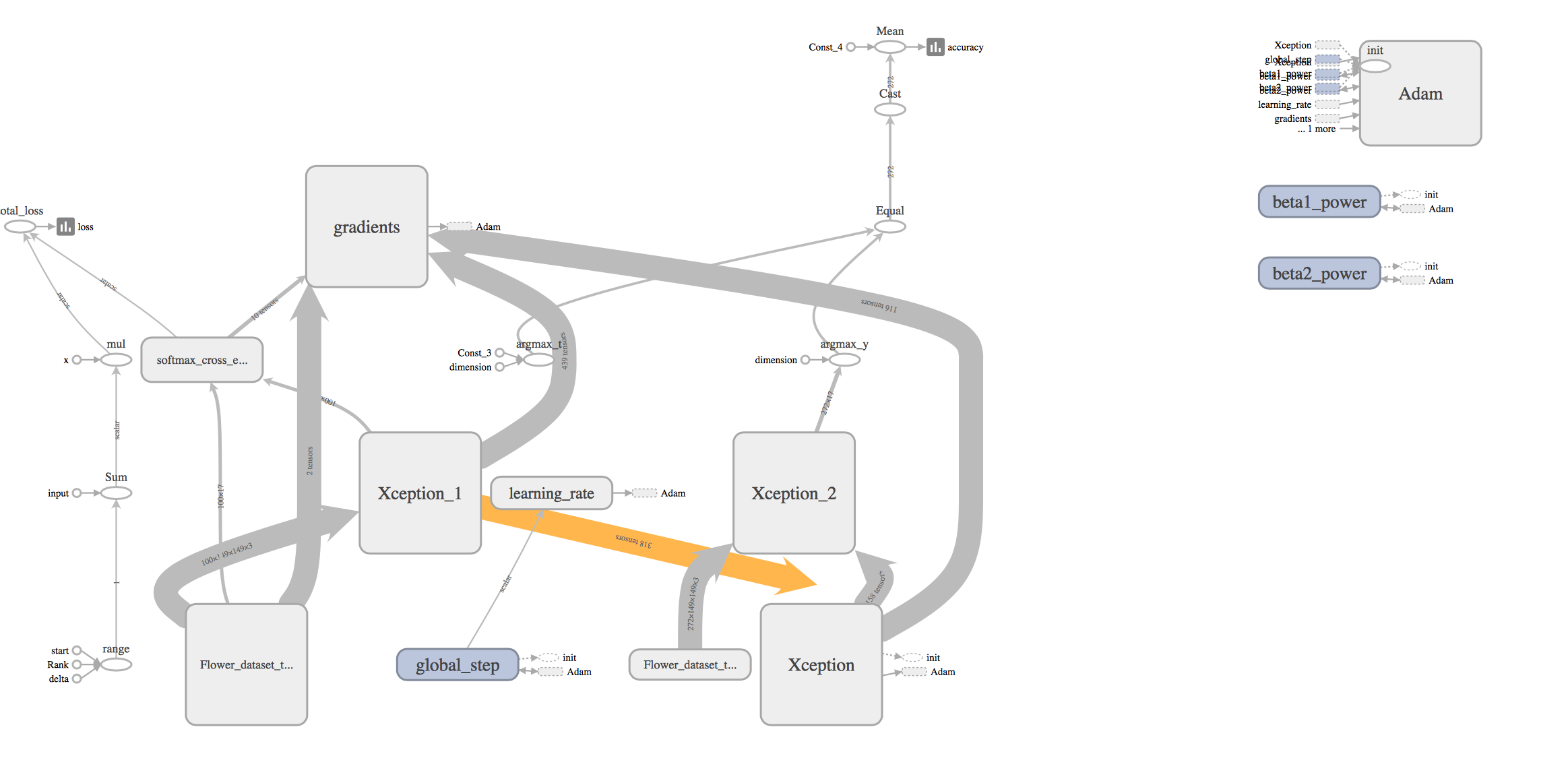
肝心のXceptionモデルの中身を展開してみると、こんな感じです。
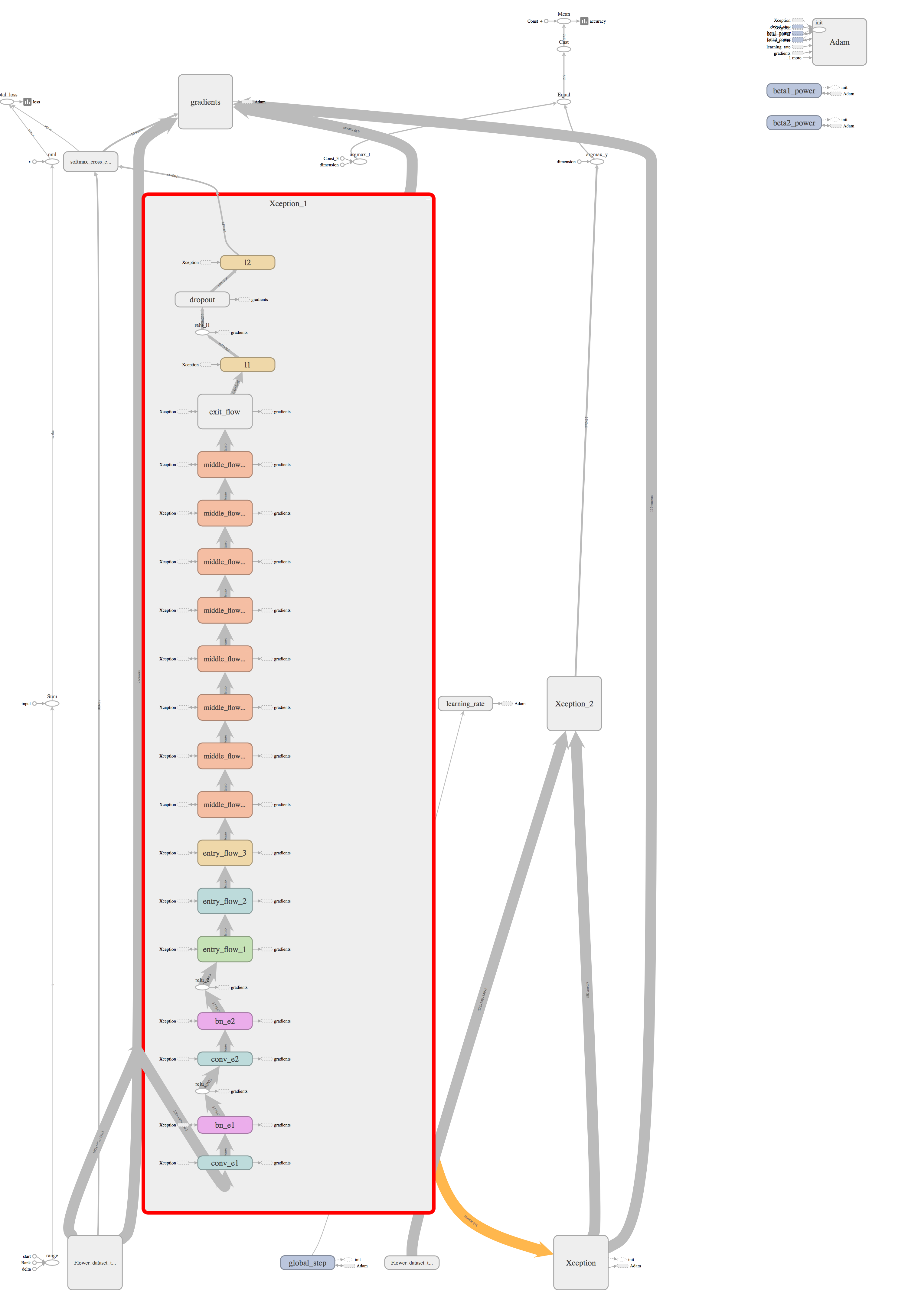
モジュールで小分けにして繋げたので、かなり見やすいと思います。
ちなみにentry_flow_1を展開すると、
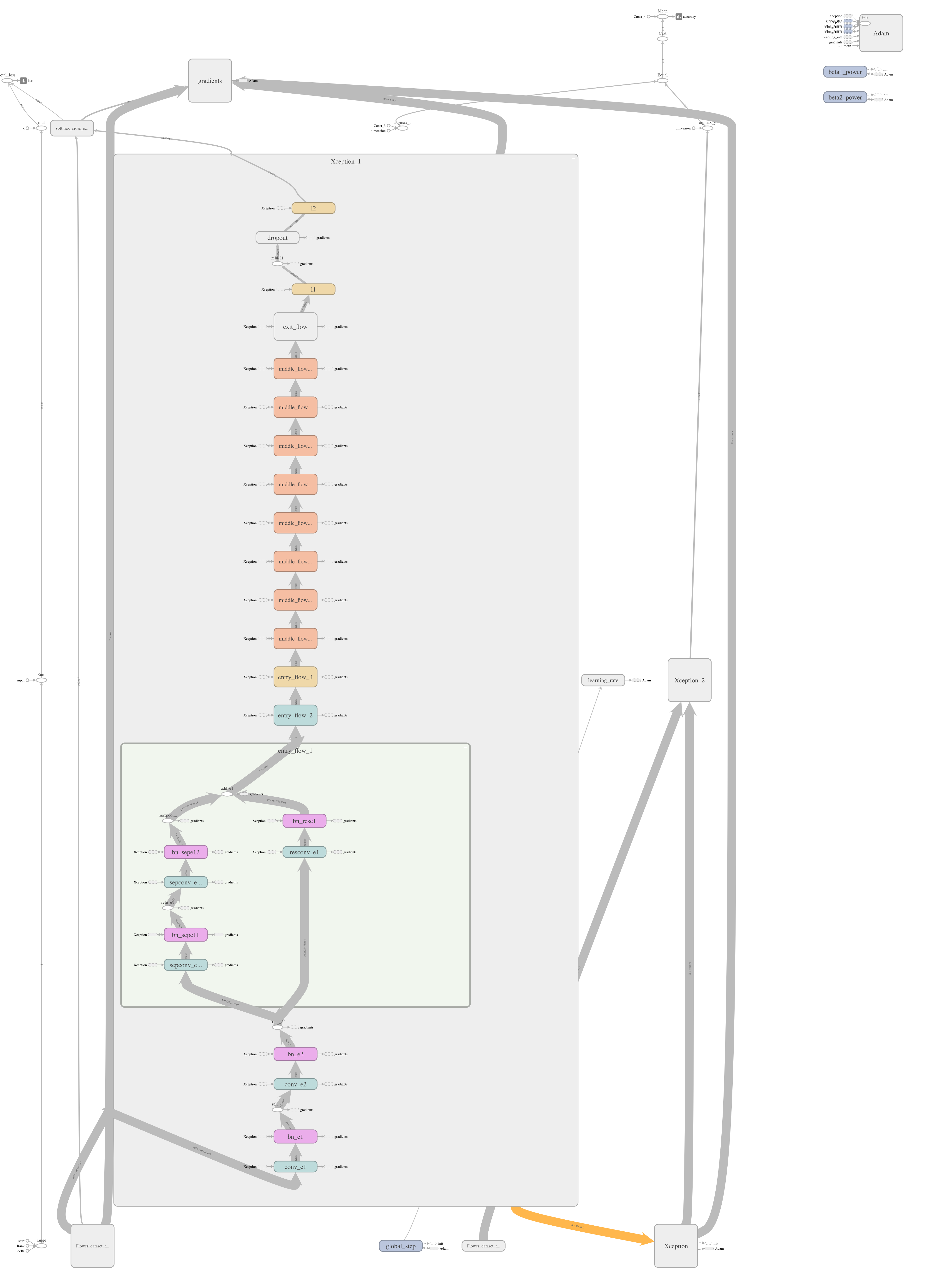
となり、論文の図と同じ感じになっていますね。
loss/accuracy曲線はこんな感じです。
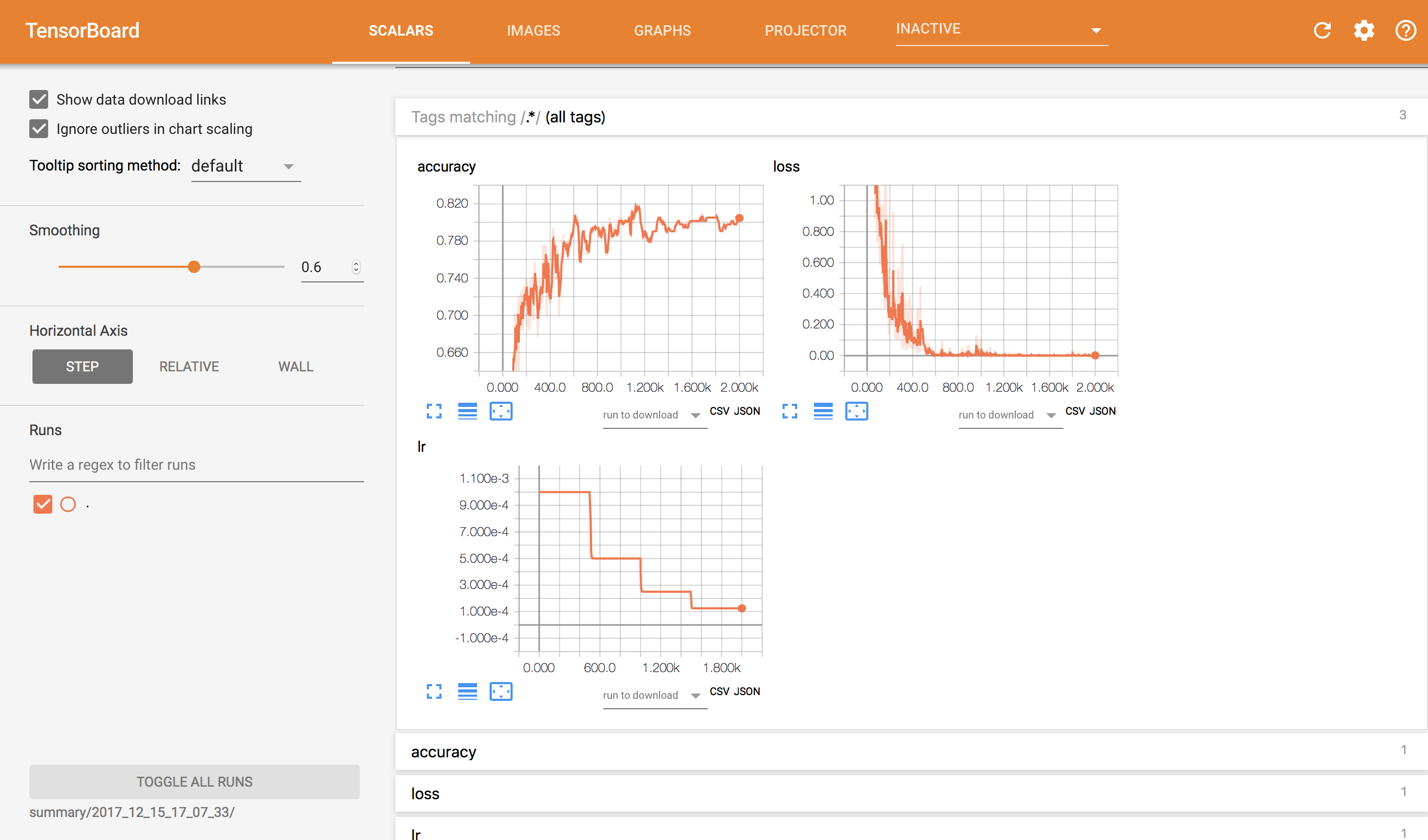
最終ステップでtest accuracy=0.805147となりました。画像サイズを変更してしまっているので、Xceptionの性能を最大限引き出した結果になっているかどうかは判断できませんね。。
最後の全結合層の1層目出力を可視化してみると、こんな感じになりました。
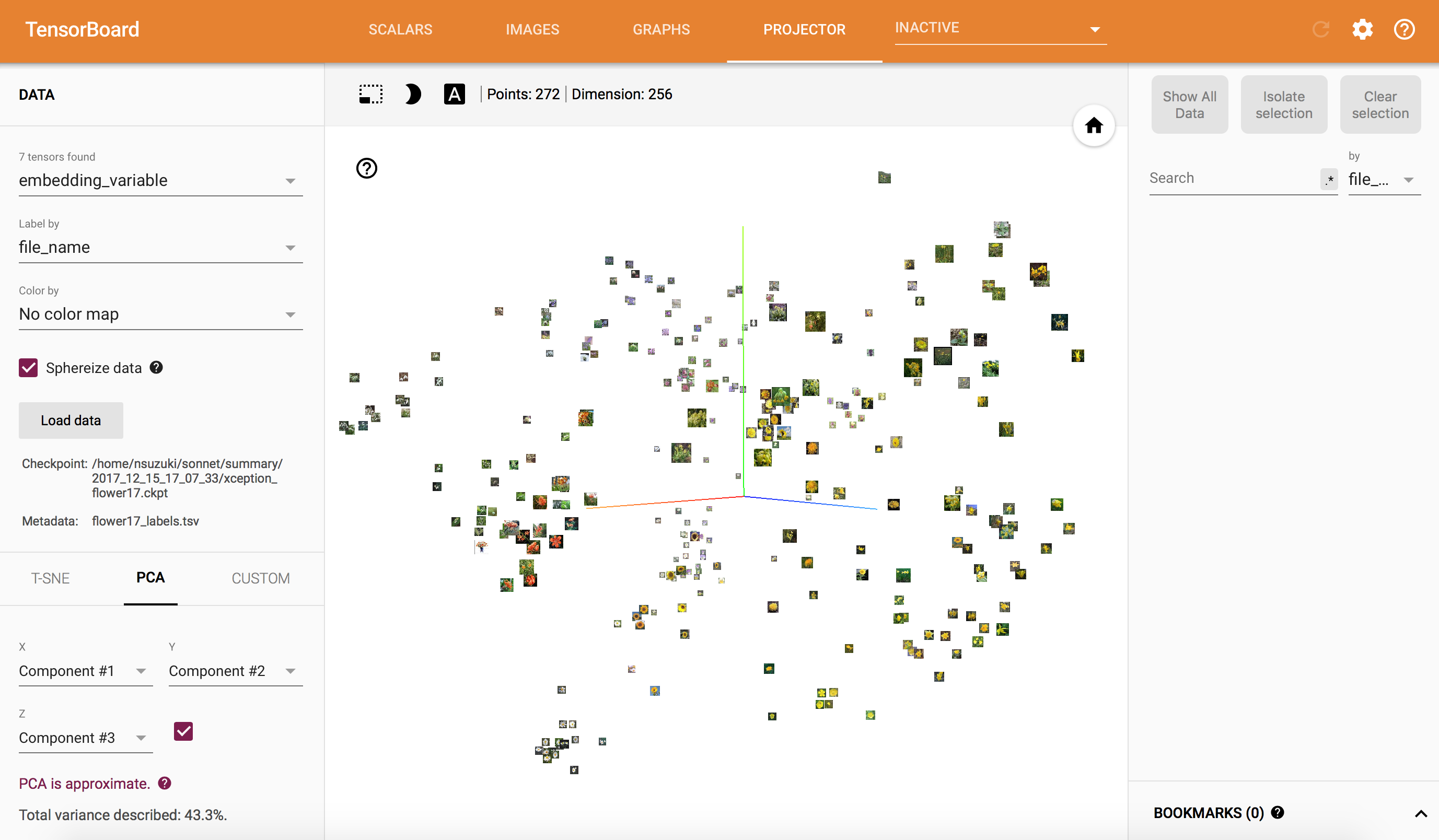
ぱっと見、似た色の花が集まっているように見えます。
もう少し拡大してみると、
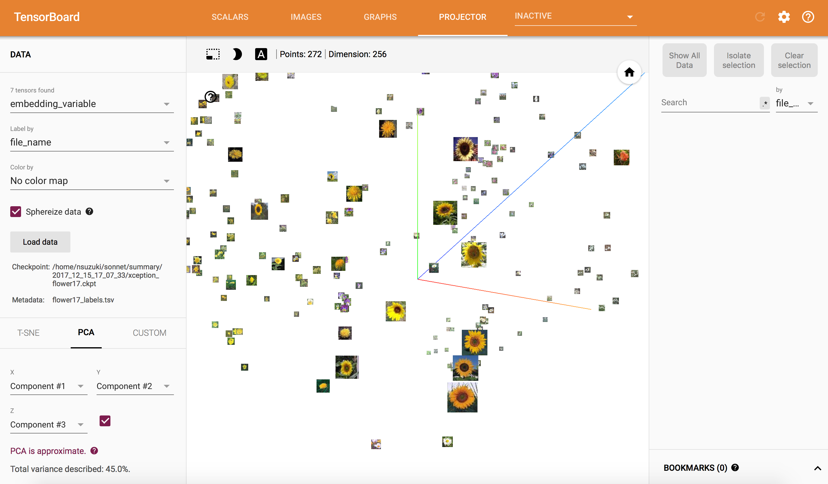
ちゃんとヒマワリが一箇所に集まっていますね!
きれいだなぁ
最後に
前回と今回で、Sonnetを使ってTensorFlow+TensorBoardをざっと一通り勉強できました(リカレントモデルに触れていないことは内緒)。Chainerばかり使ってきた私としては、割とChainer風に書けるところがあったりと、とっつきやすかったと思います。何よりTensorBoardが使えるのが大きい!
そのうちリカレントモデルにも手を出してみようと思います。。