ガウス過程 from Scratch Non-Gaussianな尤度によるガウス過程

今までに執筆した「ガウス過程 from Scratch」と「ガウス過程 from Scratch MCMCと勾配法によるハイパーパラメータ最適化」、「ガウス過程 from Scratch コレスキー分解による高速化」では、　ガウス過程(Gaussian Process) をゼロから実装しハイパーパラメータの最適化や計算の高速化を行いました。

通常のガウス過程では、関数 $\mathbf{f}$ と出力 $\mathbf{y}$　の関係 $P(\mathbf{y}|\mathbf{f})$ がガウス分布 $\mathbb{N}(\mathbf{f},\sigma^2\mathbf{I})$
に従うという前提のもと、出力を計算していました。

今回の記事では、尤度 $P(\mathbf{y}|\mathbf{f})$ がコーシー分布に従う場合を考え、データに予期しない外れ値が含まれていてもうまく回帰できるようなモデルを実装していきます。

※注意
この記事は筆者が勉強したことをまとめて、理解を深めるために執筆しています。内容に誤り等があった場合は、コメント等でご指摘いただけると幸いです。

ガウス過程(Gaussian Process)

どんなN個の入力の集合 $(\mathbf{x_{1}},\mathbf{x_{2}},\dots,\mathbf{x_{N}})$ についても、対応する出力 $(f(\mathbf{x_{1}}),f(\mathbf{x_{2}}),\dots,f(\mathbf{x_{N}}))$ の同時分布 $p(\mathbf{f})$ が、平均 $\mathbf{u}$ と $K_{n{n'}}=k(\mathbf{x_n},\mathbf{x_{n'}})$ を要素とする共分散行列 $\mathbf{K}$ のガウス分布 $\mathbb{N}(\mathbf{u},\mathbf{K})$ に従うとき、 $\mathbf{f}$ は ガウス過程(Gaussian Process) に従うと言います。

\mathbf{f}\sim \textrm{GP}(\mathbf{u},k(\mathbf{x},\mathbf{x'}))

ガウス過程は，ある$\mathbf{x}$に対してスカラー$f(\mathbf{x})$を返すのではなく，$\mathbf{x}$における$f(\mathbf{x})$が従う正規分布の平均と分散を出力します。

したがって、ガウス過程ではある予測に対する信頼度を表現することができます。下図は、ガウス過程を用いて目的関数を回帰した図になります。緑色の点が学習用データで、赤い線が平均値、水色の領域は全体の95%の信頼区間を表しています。

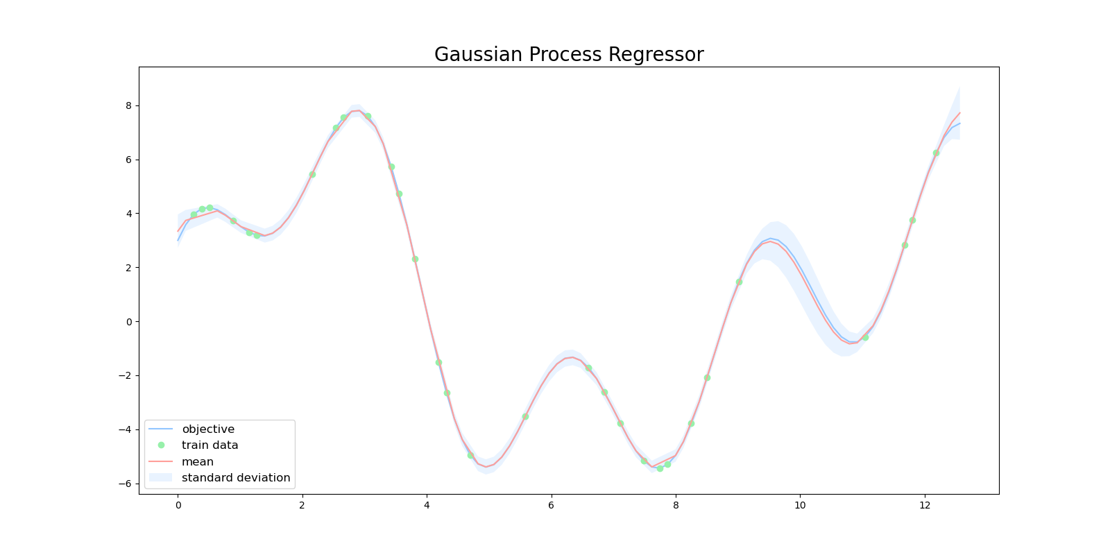
$x=10$ 周辺に注目すると、この区間では訓練データが少ないため、ガウス過程の出力も自信がない(分散が大きい)ものになっています。

一般的に観測する $y$ にはノイズがのっていることが多いので、

y = f(\mathbf{x})+\epsilon

\epsilon\sim \mathbb{N}(0,\sigma^2)

とするのが自然です。

ノイズを考慮した上でのガウス過程は、 $K_{n{n'}}=k(\mathbf{x_n},\mathbf{x_{n'}})$ を要素とする共分散行列 $\mathbf{K}$ の対角成分に、 $\sigma^2$　を足したものとして表現できます。

k'(\mathbf{x_n},\mathbf{x_{n'}})=k(\mathbf{x_n},\mathbf{x_{n'}})+\sigma^2\delta(n,n')

詳しい解説は前回の記事を参照してください。

楕円スライスサンプリング(Elliptical Sampling)

楕円スライスサンプリング(Elliptical Sampling) とは、 マルコフ連鎖モンテカルロ法(Markov chain Monte Carlo method、以下MCMC) のアルゴリズムの一つで事後分布からガウス過程を効率的にサンプリングすることができます。

$\mathbf{f}$ がガウス過程 $\textrm{GP}(\mathbf{0},\mathbf{K})$ に従っているとき、新たな提案分布 $\mathbf{f'}$ を次のように作ります。

\mathbf{f}\sim\textrm{GP}(\mathbf{0},\mathbf{K})

\mathbf{f'}=\mathbf{f}\cos\theta+\mathbf{\boldsymbol\nu}\sin\theta

\boldsymbol\nu\sim\mathbb{N}(\mathbf{0},\mathbf{K})

\theta\sim\textrm{Uni}(0,2\pi)

このとき提案分布 $\mathbf{f'}$ は

\begin{align}
\mathbb{E}[\mathbf{f'}]&=\mathbb{E}[\mathbf{f}]\cos\theta+\mathbb{E}[\mathbf{\boldsymbol\nu}]\sin\theta\\
&=\mathbf{0}+\mathbf{0}=\mathbf{0}
\end{align}

\begin{align}
\mathbb{V}[\mathbf{f'}]&=\mathbb{V}[\mathbf{f}]\cos^2\theta+\mathbb{V}[\mathbf{\boldsymbol\nu}]\sin^2\theta\\
&=\mathbf{K}(\cos^2\theta+\sin^2\theta)=\mathbf{K}
\end{align}

となりますので、 $\mathbf{f}$と同じ分布 $\mathbb{N}(0,\mathbf{K})$ を持ちます。

提案分布 $\mathbf{f'}$ に対して、尤度 $L=P(\mathbf{y}|\mathbf{f})P(\mathbf{f})$ を計算し、事前に定めた尤度の閾値 $\rho\sim\textrm{Uni}(0,L)$ よりも大きければacceptし、小さければrejectをして提案分布 $\mathbf{f'}$ をもう一度サンプリングします。

さらに、探索を効率的に行うために $\theta$ の範囲を探索するごとに狭めていきます。

楕円サンプリングを実装していきます。実際には簡単のため尤度　$L=P(\mathbf{y}|\mathbf{f})P(\mathbf{f})$　ではなくログ尤度 $\log(L)=\log(P(\mathbf{y}|\mathbf{f}))+\log(P(\mathbf{f}))$ を計算するので閾値の作り方も $L × \textrm{Uni}(0,1)$ から $\log(L) + \log(\textrm{Uni}(0,1))$ に変更されます。

import numpy as np


def elliptical(f, log_likelihood, L):
    """elipitical sampling

    f is Gaussian Process
    f ~ N(0, K)

    Args:
        f : target distribution
        log_likelihood : log likelihood of f
        L : triangle matrix of K

    """
    rho = log_likelihood(f) + np.log(np.random.uniform(0, 1))
    nu = np.dot(L, np.random.randn(len(f)))

    theta = np.random.uniform(0, 2 * np.pi)
    st, ed = theta - 2 * np.pi, theta

    while True:
        f = f * np.cos(theta) + nu * np.sin(theta)
        if log_likelihood(f) > rho:
            return f, log_likelihood(f)
        else:
            if theta > 0:
                ed = theta
            elif theta < 0:
                st = theta
            else:
                raise IOError('Slice sampling shrunk to the current position.')
            theta = np.random.uniform(st, ed)

$\boldsymbol\nu\sim\mathbb{N}(\mathbf{0},\mathbf{K})$ のサンプリングの仕方にはコレスキー分解を用いています。 $\mathbf{K}$ がガウス過程のカーネル行列のとき、

\mathbf{L}=\textrm{Cholesky}(\mathbf{K})

\mathbf{z}\sim\mathbb{N}(\mathbf{0},\mathbf{I})

\boldsymbol\nu=\mathbf{L}\mathbf{z}

とすることで、 $\mathbb{N}(\mathbf{0},\mathbf{K})$ からサンプリングすることができます。

実際に、

\begin{align}
\textrm{P}(\mathbf{z})&\propto\exp(-\frac{1}{2}\mathbf{z}^{\top}\mathbf{I}\mathbf{z})\\
&=\exp(-\frac{1}{2}\boldsymbol\nu^{\top}(\mathbf{L}^{-1})^{\top}\mathbf{I}\mathbf{L}^{-1}\boldsymbol\nu)\\
&=\exp(-\frac{1}{2}\boldsymbol\nu^{\top}(\mathbf{L}\mathbf{L}^{\top})^{-1}\boldsymbol\nu)\\
&=\exp(-\frac{1}{2}\boldsymbol\nu^{\top}(\mathbf{K})^{-1}\boldsymbol\nu)
\end{align}

となりますので、このサンプリング手法は成り立ちます。

ガウス過程と尤度

今回の記事では、目的関数として次のような三角関数の重ね合わせに、ベルヌーイ分布からのサンプルがランダムに加わった関数を考えていきます。この関数を端的に表現すると、稀に(確率0.05で)外れ値が加わって観測される関数です。

f(x)=2\sin(x)+3\cos(2x)+5\sin(\frac{2}{3}x)+10\epsilon

\epsilon\sim\textrm{Bi}(1,0.05)

実装においては、毎回同じサンプルが得られるように事前にseedを固定しておきます。

def objective(x):
    r = np.random.RandomState(2022)
    return 2 * np.sin(x) + 3 * np.cos(2 * x) + 5 * np.sin(2 / 3 * x) + 10 * \
        r.binomial(1, 0.05, len(x))

通常のガウス過程では、関数 $\mathbf{f}$ と出力 $\mathbf{y}$　の関係 $P(\mathbf{y}|\mathbf{f})$ がガウス分布 $\mathbb{N}(\mathbf{f},\sigma^2\mathbf{I})$
に従うという前提のもと出力を計算しています。

\mathbf{f}\sim\mathbb{N}(\mathbf{0},\mathbf{K})

y=f(\mathbf{x})+\epsilon

\epsilon\sim\mathbb{N}(\mathbf{0},\sigma^2\mathbf{I})

\textrm{P}(\mathbf{y}|\mathbf{f})=\mathbb{N}(\mathbf{f},\sigma^2\mathbf{I})

したがって、ガウス過程の尤度とログ尤度は次のように計算できます。計算の途中でガウス分布の正規化定数等は適宜省略していっています。

\begin{align}
L&=\textrm{P}(\mathbf{y}|\mathbf{f})\textrm{P}(\mathbf{f})\\
&=\mathbb{N}(\mathbf{f},\sigma^2\mathbf{I})\mathbb{N}(\mathbf{0},\mathbf{K})
\end{align}

\begin{align}
\log(L)&=\log(\textrm{P}(\mathbf{y}|\mathbf{f}))+\log(\textrm{P}(\mathbf{f}))\\
&\propto-\frac{1}{2}(\mathbf{y}-\mathbf{f})^{\top}(\sigma^2\mathbf{I})^{-1}(\mathbf{y}-\mathbf{f})-\frac{1}{2}\mathbf{f}^{\top}\mathbf{K}^{-1}\mathbf{f}
\end{align}

計算したログ尤度を用いて目的関数を回帰するプログラムを実装します。ガウス過程の事後分布からのサンプリングには楕円サンプリングを用います。

import numpy as np
import matplotlib.pyplot as plt
from tqdm import tqdm
from elliptical import elliptical
plt.style.use('seaborn-pastel')


def objective(x):
    r = np.random.RandomState(2022)
    return 2 * np.sin(x) + 3 * np.cos(2 * x) + 5 * np.sin(2 / 3 * x) + 10 * \
        r.binomial(1, 0.05, len(x))


def rbf(x, x_prime, theta_1, theta_2):
    """RBF Kernel

    Args:
        x (float): data
        x_prime (float): data
        theta_1 (float): hyper parameter
        theta_2 (float): hyper parameter
    """

    return theta_1 * np.exp(-1 * (x - x_prime)**2 / theta_2)


# Radiant Basis Kernel
def kernel(x, x_prime, noise):
    theta_3 = 1e-6
    # delta function
    if noise:
        delta = theta_3
    else:
        delta = 0
    return rbf(x, x_prime, theta_1=1.0, theta_2=1.0) + delta


def plot_gpr(x, y, f_posterior):
    plt.figure(figsize=(16, 8))
    plt.title('Cauchy', fontsize=20)
    plt.plot(x, y, 'x', label='objective')

    for i in range(f_posterior.shape[1]):
        plt.plot(x, f_posterior[:, i])
    plt.savefig('gaussian.png')


def gpr(x, y, kernel, n_iter=100):
    N = len(x)

    K = np.zeros((N, N))
    for x_idx in range(N):
        for x_prime_idx in range(N):
            K[x_idx, x_prime_idx] = kernel(
                x[x_idx], x[x_prime_idx], x_idx == x_prime_idx)

    K_inv = np.linalg.inv(K)
    I_inv = np.linalg.inv(1e-6 * np.eye(len(y)))
    L_ = np.linalg.cholesky(K)

    # Normalization
    y_mean = np.mean(y)
    y_std = np.std(y)
    y = (y - y_mean) / y_std

    def log_marginal_likelihood(y, f):
        return - 0.5 * np.dot(y - f, np.dot(I_inv, y - f)) - \
            0.5 * np.dot(f, np.dot(K_inv, f))

    burn_in = 50
    n_samples = n_iter - burn_in
    assert n_iter > burn_in

    f = np.dot(L_, np.random.randn(N))
    f_posterior = np.zeros((f.shape[0], n_samples))
    for i in tqdm(range(n_iter)):

        sampling = True
        while sampling:
            try:
                f, _ = elliptical(f, lambda f: log_marginal_likelihood(y, f), L_)
                sampling = False
            except IOError:
                # print('Slice sampling shrunk to the current position. Retry sampling ...')
                sampling = True

        if i >= burn_in:
            f_posterior[:, i - burn_in] = f * y_std + y_mean

    return f_posterior


if __name__ == "__main__":
    n = 100
    x = np.linspace(0, 4 * np.pi, n)
    y = objective(x)

    f_posterior = gpr(x, y, kernel)
    plot_gpr(x, y, f_posterior)

計算と実装の簡単化のためにガウス過程の平均はデータを正規化することで0にしています。

    # Normalization
    y_mean = np.mean(y)
    y_std = np.std(y)
    y = (y - y_mean) / y_std

楕円スライスサンプリングを実行しているのは以下の箇所になります。一般的なMCMCによるサンプリングでは、前半のサンプリングは burn-in(慣らし運転) として棄却するので、今回も実装も例に倣い最初の50個のサンプルを棄却しています。

    burn_in = 50
    n_samples = n_iter - burn_in
    assert n_iter > burn_in

    f = np.dot(L_, np.random.randn(N))
    f_posterior = np.zeros((f.shape[0], n_samples))
    for i in tqdm(range(n_iter)):

        sampling = True
        while sampling:
            try:
                f, _ = elliptical(f, lambda f: log_marginal_likelihood(y, f), L_)
                sampling = False
            except IOError:
                # print('Slice sampling shrunk to the current position. Retry sampling ...')
                sampling = True

        if i >= burn_in:
            f_posterior[:, i - burn_in] = f * y_std + y_mean

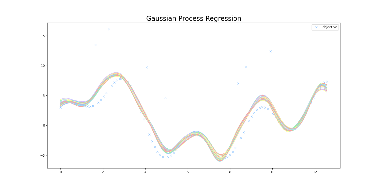
このプログラムを実行すると、次のような結果が得られます。目的関数に存在する外れ値に影響されてうまく回帰ができていません。

コーシー分布によるロバストなガウス過程

コーシー分布は次のような確率密度関数で表されます。

\textrm{P}(x|x_0,\gamma)=\frac{\gamma}{\pi\{(x-x_0)+\gamma^2\}}

x_0\in\mathbb{R}

\gamma>0

正規分布に比べてコーシー分布の方は、0から遠いところでの減衰が遅く、裾の厚い分布(heavy tailed)になります。正規分布の確率密度関数が指数的に減衰するのに対し、コーシー分布は $x^2$ 程度の減衰のため、減衰が遅くなります。

[出典]コーシー分布の定義と性質とその証明

一つ前のセクションで実装したガウス過程は、ガウス分布に誤差が含まれて観測されるというモデルになっているので、今回のような大きな外れ値がある場合はガウス分布が外れ値を説明するためにガウス分布の平均が外れ値側に偏って推定されてしまいます。

これに対して、誤差の分布 $\textrm{P}(\mathbf{y}|\mathbf{f})$ にコーシー分布を用いることで、目的関数に外れ値が含まれていてもコーシー分布の裾の厚さで外れ値を説明することができます。

このとき $\mathbf{f}$ の事後分布 $P(\mathbf{f}|\mathbf{y})$ は

\begin{align}
P(\mathbf{f}|\mathbf{y})&\propto P(\mathbf{y}|\mathbf{f})P(\mathbf{f})\\
&=(\prod_{n=1}^{N}\textrm{Cauchy}(y_n|f_n,\gamma))\mathbb{N}(\mathbf{0},\mathbf{K})\\
&\propto (\prod_{n=1}^{N}\frac{\gamma}{\pi\{(y_n-f_n)^2+\gamma^2\}})\exp(-\frac{1}{2}\mathbf{f}^{\top}\mathbf{K}^{-1}\mathbf{f})
\end{align}

となります。計算と実装の簡単化のためログ尤度を計算すると

\begin{align}
\log P(\mathbf{y}|\mathbf{f})P(\mathbf{f})&=\log(\textrm{P}(\mathbf{y}|\mathbf{f}))+\log(\textrm{P}(\mathbf{f}))\\
&\propto -\sum_{n=1}^N\log(\gamma+\frac{(y_n-f_n)^2}{\gamma}) -\frac{1}{2}\mathbf{f}^{\top}\mathbf{K}^{-1}\mathbf{f}
\end{align}

となります。

コーシー分布を用いた尤度でガウス過程を実行するプログラムを実装します。基本的にはログ尤度の計算が変わっただけです。

import matplotlib.pyplot as plt
import numpy as np
from tqdm import tqdm
from elliptical import elliptical
plt.style.use('seaborn-pastel')


def objective(x):
    r = np.random.RandomState(2022)
    return 2 * np.sin(x) + 3 * np.cos(2 * x) + 5 * np.sin(2 / 3 * x) + 10 * \
        r.binomial(1, 0.05, len(x))


def rbf(x, x_prime, theta_1, theta_2):
    """RBF Kernel

    Args:
        x (float): data
        x_prime (float): data
        theta_1 (float): hyper parameter
        theta_2 (float): hyper parameter
    """

    return theta_1 * np.exp(-1 * (x - x_prime)**2 / theta_2)


# Radiant Basis Kernel
def kernel(x, x_prime, noise):
    theta_3 = 1e-6
    # delta function
    if noise:
        delta = theta_3
    else:
        delta = 0
    return rbf(x, x_prime, theta_1=1.0, theta_2=1.0) + delta


def plot_gpr(x, y, f_posterior):
    plt.figure(figsize=(16, 8))
    plt.title('Gaussian Process with Cauchy Distribution', fontsize=20)
    plt.plot(x, y, 'x', label='objective')

    for i in range(f_posterior.shape[1]):
        plt.plot(x, f_posterior[:, i])
    plt.legend()
    plt.savefig('cauchy.png')


def gpr(x, y, kernel, n_iter=100):
    N = len(x)

    K = np.zeros((N, N))
    for x_idx in range(N):
        for x_prime_idx in range(N):
            K[x_idx, x_prime_idx] = kernel(
                x[x_idx], x[x_prime_idx], x_idx == x_prime_idx)

    K_inv = np.linalg.inv(K)
    L_ = np.linalg.cholesky(K)

    # Normalization
    y_mean = np.mean(y)
    y_std = np.std(y)
    y = (y - y_mean) / y_std

    def log_marginal_likelihood(y, f, gamma=0.2):
        cauchy = - np.sum(np.log(gamma + (y - f)**2 / gamma))
        normal = - 0.5 * np.dot(f, np.dot(K_inv, f))
        return cauchy + normal

    burn_in = 50
    n_samples = n_iter - burn_in
    assert n_iter > burn_in

    f = np.dot(L_, np.random.randn(N))
    f_posterior = np.zeros((f.shape[0], n_samples))
    for i in tqdm(range(n_iter)):

        sampling = True
        while sampling:
            try:
                f, _ = elliptical(f, lambda f: log_marginal_likelihood(y, f), L_)
                sampling = False
            except IOError:
                # print('Slice sampling shrunk to the current position. Retry sampling ...')
                sampling = True

        if i >= burn_in:
            f_posterior[:, i - burn_in] = f * y_std + y_mean

    return f_posterior


if __name__ == "__main__":
    n = 100
    x = np.linspace(0, 4 * np.pi, n)
    y = objective(x)

    f_posterior = gpr(x, y, kernel)
    plot_gpr(x, y, f_posterior)

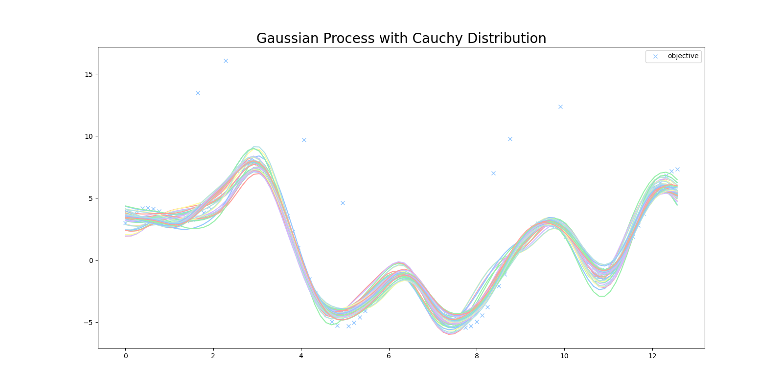
このプログラムを実行すると次のような結果が得られました。 $\textrm{P}(\mathbf{y}|\mathbf{f})$ にガウス分布を用いたときより、外れ値の影響を避けて目的関数を回帰することに成功しています。

まとめ

ガウス過程の尤度にコーシー分布を用いて目的関数を回帰するプログラムをゼロから実装してみました。

尤度に裾が厚いコーシー分布を用いることで、外れ値の影響を受けない頑健(Robust)なモデルを作ることに成功しました。

今回はコーシー分布を用いましたが、ベルヌーイ分布やポアソン分布などの他の分布を用いることで、特定の状況に適したガウス過程のモデルを作ることができます。

ここまで読んでいただきありがとうございます。

今回実装したコードは全てこちらのレポジトリにあります。

参考文献

[1] C. E. Rasmussen and C. K. I. Williams. Gaussian Processes for Machine Learning. 2006.
[2] Iain Murray, Ryan Prescott Adams, David J.C. MacKay. Elliptical slice sampling. 2009.
[3] 持橋 大地, ガウス過程と機械学習. 2019.