More than 1 year has passed since last update.

GridSearchCV HalvingGridSearchCV RandomizedSearchCV HalvingRandomSearchCV を理解する

Last updated at 2023-02-27Posted at 2023-02-27

機械学習でハイパーパラメーターチューニングといえば Optuna が柔軟なコーディングができて個人的にはお気に入りなんですが、scikit-learnのGridSearchCVとその兄弟たちの使い方を理解してみたくなったので試してみました。

データセットとその分割

回帰用データセットとして load_diabetes を用い、train_test_split を用いて教師データとテストデータに分割します。

import sklearn.datasets
from sklearn.model_selection import train_test_split

dataset = sklearn.datasets.load_diabetes()
X_train, X_test, Y_train, Y_test = train_test_split(dataset.data, dataset.target)

HistGradientBoostingRegressor

HistGradientBoostingRegressor は、非深層系機械学習モデルとして最強クラスと噂されている（？）勾配ブースティング回帰の、scikit-learnによる軽量型とのことです。

from sklearn.ensemble import HistGradientBoostingRegressor

model = HistGradientBoostingRegressor()
model.fit(X_train, Y_train)
model.score(X_test, Y_test)

0.3174338258206677

以上が、ハイパラチューニングなしでの結果となりますが、さてさて、GridSearchCV HalvingGridSearchCV RandomizedSearchCV HalvingRandomSearchCV の４つの CV (Cross Validation) 手法を用いてどのくらい改善できるでしょうか？

GridSearchCV

まずは GridSearchCV を使ってみましょう。GridSearchCV は、与えたパラメーターの全組み合わせに対して学習を行なって、ベストな学習器を発見します。

from sklearn.model_selection import GridSearchCV

parameters = dict(
    {
        "loss": ["squared_error", "absolute_error", "poisson"],
        "learning_rate": [0.2, 0.1, 0.05],
        "max_leaf_nodes": [2, 8, 32],
        "max_depth": [2, 8, 32],
        "min_samples_leaf": [2, 8, 32],
        "max_bins": [64, 128, 255],
    }
)
model = GridSearchCV(HistGradientBoostingRegressor(), parameters, cv=5, n_jobs=-1)
model.fit(X_train, Y_train)
print("R2=", model.score(X_test, Y_test))
model.best_estimator_

R2= 0.33232614171975594

少しは改善しましたね。そのベストモデルのハイパーパラメーターは次の通りです。

HistGradientBoostingRegressor(learning_rate=0.05, loss='absolute_error',
                              max_bins=128, max_depth=32, max_leaf_nodes=32,
                              min_samples_leaf=8)

以上のGridSearchCVの詳細な結果は次のように確認できます。

import pandas as pd

pd.DataFrame(model.cv_results_)

	mean_fit_time	std_fit_time	mean_score_time	std_score_time	param_learning_rate	param_loss	param_max_bins	param_max_depth	param_max_leaf_nodes	param_min_samples_leaf	params	split0_test_score	split1_test_score	split2_test_score	split3_test_score	split4_test_score	mean_test_score	std_test_score	rank_test_score
0	0.046092	0.001038	0.003924	0.000962	0.2	squared_error	64	2	2	2	{'learning_rate': 0.2, 'loss': 'squared_error'...	0.510208	0.403854	0.419810	0.316751	0.504165	0.430958	0.071473	344
1	0.047879	0.004027	0.003343	0.000078	0.2	squared_error	64	2	2	8	{'learning_rate': 0.2, 'loss': 'squared_error'...	0.534582	0.414399	0.412338	0.323632	0.506877	0.438365	0.075322	186
2	0.044900	0.001714	0.003401	0.000135	0.2	squared_error	64	2	2	32	{'learning_rate': 0.2, 'loss': 'squared_error'...	0.554374	0.445249	0.369375	0.315602	0.467517	0.430423	0.082305	357
3	0.080580	0.007363	0.004332	0.001743	0.2	squared_error	64	2	8	2	{'learning_rate': 0.2, 'loss': 'squared_error'...	0.425588	0.450360	0.362742	0.284584	0.443050	0.393265	0.062492	596
4	0.069854	0.004283	0.003402	0.000314	0.2	squared_error	64	2	8	8	{'learning_rate': 0.2, 'loss': 'squared_error'...	0.495745	0.401067	0.347681	0.262674	0.469976	0.395429	0.084328	590
...	...	...	...	...	...	...	...	...	...	...	...	...	...	...	...	...	...	...	...
724	0.145537	0.009800	0.003565	0.000112	0.05	poisson	255	32	8	8	{'learning_rate': 0.05, 'loss': 'poisson', 'ma...	0.536389	0.477789	0.396651	0.323495	0.397866	0.426438	0.073521	427
725	0.102996	0.001280	0.003632	0.000067	0.05	poisson	255	32	8	32	{'learning_rate': 0.05, 'loss': 'poisson', 'ma...	0.593431	0.462807	0.358350	0.390233	0.410602	0.443085	0.082488	120
726	0.565122	0.031652	0.005548	0.002976	0.05	poisson	255	32	32	2	{'learning_rate': 0.05, 'loss': 'poisson', 'ma...	0.474264	0.399449	0.398237	0.223435	0.258033	0.350683	0.094539	679
727	0.378403	0.015974	0.004088	0.000225	0.05	poisson	255	32	32	8	{'learning_rate': 0.05, 'loss': 'poisson', 'ma...	0.486323	0.485514	0.333050	0.337733	0.327221	0.393968	0.075152	595
728	0.099264	0.013943	0.003375	0.000581	0.05	poisson	255	32	32	32	{'learning_rate': 0.05, 'loss': 'poisson', 'ma...	0.593431	0.462807	0.358350	0.390233	0.410602	0.443085	0.082488	120

729 rows × 19 columns

今回、６種類のハイパーパラメータがそれぞれ３個の値を持っていたので 3 * 3 * 3 * 3 * 3 * 3 = 729 ということで、累計 729 個の機械学習モデルを生成したということで計算は合っていますね。

どのようなハイパラを探索していたか確認してみましょう。

pd.DataFrame(model.cv_results_["params"])

	learning_rate	loss	max_bins	max_depth	max_leaf_nodes	min_samples_leaf
0	0.20	squared_error	64	2	2	2
1	0.20	squared_error	64	2	2	8
2	0.20	squared_error	64	2	2	32
3	0.20	squared_error	64	2	8	2
4	0.20	squared_error	64	2	8	8
...	...	...	...	...	...	...
724	0.05	poisson	255	32	8	8
725	0.05	poisson	255	32	8	32
726	0.05	poisson	255	32	32	2
727	0.05	poisson	255	32	32	8
728	0.05	poisson	255	32	32	32

729 rows × 6 columns

次のように結合してみます。

cv_results_df = pd.concat(
    [pd.DataFrame(model.cv_results_), pd.DataFrame(model.cv_results_["params"])], axis=1
)
cv_results_df

	mean_fit_time	std_fit_time	mean_score_time	std_score_time	param_learning_rate	param_loss	param_max_bins	param_max_depth	param_max_leaf_nodes	param_min_samples_leaf	...	split4_test_score	mean_test_score	std_test_score	rank_test_score	learning_rate	loss	max_bins	max_depth	max_leaf_nodes	min_samples_leaf
0	0.046092	0.001038	0.003924	0.000962	0.2	squared_error	64	2	2	2	...	0.504165	0.430958	0.071473	344	0.20	squared_error	64	2	2	2
1	0.047879	0.004027	0.003343	0.000078	0.2	squared_error	64	2	2	8	...	0.506877	0.438365	0.075322	186	0.20	squared_error	64	2	2	8
2	0.044900	0.001714	0.003401	0.000135	0.2	squared_error	64	2	2	32	...	0.467517	0.430423	0.082305	357	0.20	squared_error	64	2	2	32
3	0.080580	0.007363	0.004332	0.001743	0.2	squared_error	64	2	8	2	...	0.443050	0.393265	0.062492	596	0.20	squared_error	64	2	8	2
4	0.069854	0.004283	0.003402	0.000314	0.2	squared_error	64	2	8	8	...	0.469976	0.395429	0.084328	590	0.20	squared_error	64	2	8	8
...	...	...	...	...	...	...	...	...	...	...	...	...	...	...	...	...	...	...	...	...	...
724	0.145537	0.009800	0.003565	0.000112	0.05	poisson	255	32	8	8	...	0.397866	0.426438	0.073521	427	0.05	poisson	255	32	8	8
725	0.102996	0.001280	0.003632	0.000067	0.05	poisson	255	32	8	32	...	0.410602	0.443085	0.082488	120	0.05	poisson	255	32	8	32
726	0.565122	0.031652	0.005548	0.002976	0.05	poisson	255	32	32	2	...	0.258033	0.350683	0.094539	679	0.05	poisson	255	32	32	2
727	0.378403	0.015974	0.004088	0.000225	0.05	poisson	255	32	32	8	...	0.327221	0.393968	0.075152	595	0.05	poisson	255	32	32	8
728	0.099264	0.013943	0.003375	0.000581	0.05	poisson	255	32	32	32	...	0.410602	0.443085	0.082488	120	0.05	poisson	255	32	32	32

729 rows × 25 columns

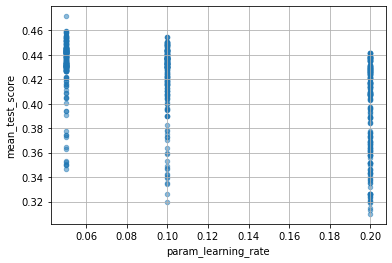
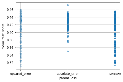
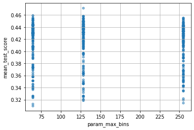
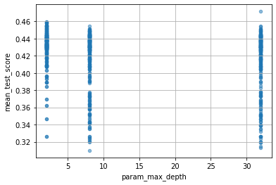
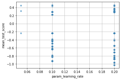
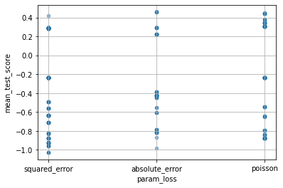
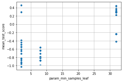
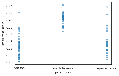
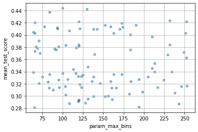
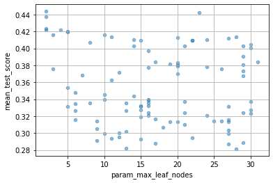
次のようにすれば、各パラメーターが性能にどのくらい影響したかを確認できます。ただし、ここでいう mean_test_score は、ややこしいのですが、(X_test, Y_test) に対するscoreではなくて、(X_train, Y_train) を cv=5 として分割したときの test_score の平均ということになります。

for col in cv_results_df.columns:
    if col[:6] == "param_":
        cv_results_df.plot(col, "mean_test_score", kind="scatter", alpha=0.5, grid=True)

HalvingGridSearchCV

次は HalvingGridSearchCV です。これは、GridSearchCV と同様に全組み合わせを探索した後に、スコアの高かった組み合わせを取り出し、上位のモデルに対してより多い resource を与えて再学習を行うという操作を繰り返します。

上位いくつの組み合わせを選ぶかは factor というパラメーターで調整できます（たとえば factor=2 とすれば上位 1/2 のモデルが選択されます）。

resource とは何か、というのは base となる estimator によって変わるらしく、GradientBoosting のようなアンサンブル学習器なら n_estimators になるようです。

from sklearn.experimental import enable_halving_search_cv
from sklearn.model_selection import HalvingGridSearchCV

parameters = dict(
    {
        "loss": ["squared_error", "absolute_error", "poisson"],
        "learning_rate": [0.2, 0.1, 0.05],
        "max_leaf_nodes": [2, 8, 32],
        "max_depth": [2, 8, 32],
        "min_samples_leaf": [2, 8, 32],
        "max_bins": [64, 128, 255],
    }
)
model = HalvingGridSearchCV(
    HistGradientBoostingRegressor(), parameters, cv=5, n_jobs=-1
)
model.fit(X_train, Y_train)
print("R2=", model.score(X_test, Y_test))
model.best_estimator_

R2= 0.45168983833467624

お、けっこう性能が向上しましたね。

HistGradientBoostingRegressor(learning_rate=0.2, loss='absolute_error',
                              max_bins=64, max_depth=2, max_leaf_nodes=2,
                              min_samples_leaf=2)

クロスバリデーションの詳細は次の通りです。 iter=0 では単純な GridSearchCV と同じ 3 * 3 * 3 * 3 * 3 * 3 = 729 個のモデルが学習され、上位 1/factor 個のモデルが選択され、より多い resource で再学習されるということを繰り返します。

cv_results_df = pd.concat(
    [pd.DataFrame(model.cv_results_), pd.DataFrame(model.cv_results_["params"])], axis=1
)
cv_results_df

	iter	n_resources	mean_fit_time	std_fit_time	mean_score_time	std_score_time	param_learning_rate	param_loss	param_max_bins	param_max_depth	...	split3_train_score	split4_train_score	mean_train_score	std_train_score	learning_rate	loss	max_bins	max_depth	max_leaf_nodes	min_samples_leaf
0	0	10	0.073146	0.035112	0.008809	0.005226	0.2	squared_error	64	2	...	0.999956	0.999969	0.999855	2.293240e-04	0.20	squared_error	64	2	2	2
1	0	10	0.036513	0.015857	0.007700	0.005450	0.2	squared_error	64	2	...	0.000000	0.000000	0.000000	0.000000e+00	0.20	squared_error	64	2	2	8
2	0	10	0.048790	0.014432	0.005903	0.003738	0.2	squared_error	64	2	...	0.000000	0.000000	0.000000	0.000000e+00	0.20	squared_error	64	2	2	32
3	0	10	0.117461	0.019852	0.007106	0.005961	0.2	squared_error	64	2	...	1.000000	1.000000	1.000000	2.120790e-08	0.20	squared_error	64	2	8	2
4	0	10	0.052612	0.004677	0.004469	0.002280	0.2	squared_error	64	2	...	0.000000	0.000000	0.000000	0.000000e+00	0.20	squared_error	64	2	8	8
...	...	...	...	...	...	...	...	...	...	...	...	...	...	...	...	...	...	...	...	...	...
1075	3	270	0.093966	0.012485	0.007732	0.006771	0.2	poisson	128	8	...	0.633315	0.616487	0.614829	3.458072e-02	0.20	poisson	128	8	2	32
1076	3	270	0.136020	0.012811	0.003038	0.000059	0.2	poisson	128	2	...	0.793938	0.759121	0.779202	2.804673e-02	0.20	poisson	128	2	32	32
1077	3	270	0.145647	0.047377	0.005804	0.003204	0.2	poisson	128	2	...	0.793938	0.759121	0.779202	2.804673e-02	0.20	poisson	128	2	8	32
1078	3	270	0.129800	0.026974	0.003437	0.000220	0.2	poisson	64	32	...	0.876194	0.870592	0.870216	1.899521e-02	0.20	poisson	64	32	32	32
1079	3	270	0.129445	0.042735	0.004040	0.001468	0.05	poisson	255	32	...	0.723216	0.705591	0.705248	3.103351e-02	0.05	poisson	255	32	32	32

1080 rows × 34 columns

各パラメータが性能にどのような影響を与えたかは次のようにして見られます。

for col in cv_results_df.columns:
    if col[:6] == "param_":
        cv_results_df.plot(col, "mean_test_score", kind="scatter", alpha=0.5, grid=True)

より多い resource で再学習する分、性能が向上するというのは良いとしても、ハイパラの探索範囲は GridSearchCV と変わらないということですね。

RandomizedSearchCV

次は RandomizedSearchCV です。これは、名前から想像できる通り、指定したハイパーパラメーターの範囲をランダムにサーチします。反復回数は n_iter=100 のように指定します。

from scipy.stats import randint, uniform
from sklearn.model_selection import RandomizedSearchCV

parameters = dict(
    {
        "loss": ["squared_error", "absolute_error", "poisson"],
        "learning_rate": uniform(0.2, 0.05),
        "max_leaf_nodes": randint(2, 32),
        "max_depth": randint(2, 32),
        "min_samples_leaf": randint(2, 32),
        "max_bins": randint(64, 255),
    }
)
model = RandomizedSearchCV(
    HistGradientBoostingRegressor(), parameters, cv=5, n_jobs=-1, n_iter=100
)
model.fit(X_train, Y_train)
print("R2=", model.score(X_test, Y_test))
model.best_estimator_

R2= 0.44293642952519996

今回、GridSearchCVよりは改善しましたが、HalvingGridSearchCVには負けた、という形ですね。

HistGradientBoostingRegressor(learning_rate=0.2401623294668279,
                              loss='absolute_error', max_bins=100, max_depth=27,
                              max_leaf_nodes=2, min_samples_leaf=31)

結果の詳細です。

cv_results_df = pd.concat(
    [pd.DataFrame(model.cv_results_), pd.DataFrame(model.cv_results_["params"])], axis=1
)
cv_results_df

	mean_fit_time	std_fit_time	mean_score_time	std_score_time	param_learning_rate	param_loss	param_max_bins	param_max_depth	param_max_leaf_nodes	param_min_samples_leaf	...	split4_test_score	mean_test_score	std_test_score	rank_test_score	learning_rate	loss	max_bins	max_depth	max_leaf_nodes	min_samples_leaf
0	0.366715	0.053425	0.014998	0.003574	0.230097	poisson	82	3	30	9	...	0.274491	0.323229	0.060283	70	0.230097	poisson	82	3	30	9
1	0.506211	0.144560	0.011002	0.006287	0.226155	absolute_error	173	27	5	10	...	0.428027	0.419660	0.093885	8	0.226155	absolute_error	173	27	5	10
2	0.221872	0.035509	0.012181	0.007027	0.200513	absolute_error	66	23	5	30	...	0.410435	0.419785	0.091442	7	0.200513	absolute_error	66	23	5	30
3	0.196586	0.026616	0.006464	0.003607	0.213685	squared_error	106	31	30	29	...	0.322769	0.327327	0.089463	64	0.213685	squared_error	106	31	30	29
4	0.192499	0.050251	0.007767	0.003510	0.227877	squared_error	108	5	17	19	...	0.254810	0.287950	0.057030	97	0.227877	squared_error	108	5	17	19
...	...	...	...	...	...	...	...	...	...	...	...	...	...	...	...	...	...	...	...	...	...
95	0.399913	0.010536	0.003984	0.000305	0.22602	absolute_error	170	26	15	5	...	0.436215	0.409727	0.062342	17	0.226020	absolute_error	170	26	15	5
96	0.083641	0.015314	0.003447	0.000209	0.206473	poisson	116	2	30	4	...	0.376263	0.337107	0.027581	53	0.206473	poisson	116	2	30	4
97	0.163723	0.090995	0.009293	0.004980	0.23693	poisson	194	3	13	13	...	0.285729	0.282265	0.052020	99	0.236930	poisson	194	3	13	13
98	0.551714	0.115441	0.004080	0.000183	0.233486	squared_error	159	16	29	2	...	0.315230	0.323911	0.061675	68	0.233486	squared_error	159	16	29	2
99	0.181508	0.039065	0.003228	0.000828	0.221521	squared_error	249	18	12	6	...	0.363508	0.371630	0.068751	40	0.221521	squared_error	249	18	12	6

100 rows × 25 columns

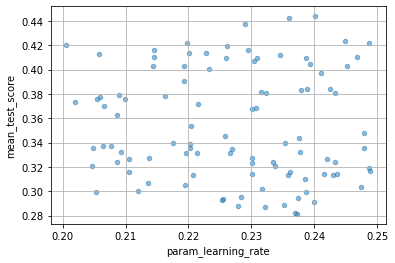
ランダムなので、最適なハイパラの値がほとんど見当がつかないような時に便利なんだろうと思います。

for col in cv_results_df.columns:
    if col[:6] == "param_":
        cv_results_df.plot(col, "mean_test_score", kind="scatter", alpha=0.5, grid=True)

HalvingRandomSearchCV

最後に、HalvingRandomSearchCVです。これは、GridSearchCVに対するHalvingGridSearchCVと同様に、RandomSearchCVに対して、上位いくつかのモデルに対してresouceを増やして再計算するというものです。

from scipy.stats import randint, uniform
from sklearn.experimental import enable_halving_search_cv
from sklearn.model_selection import HalvingRandomSearchCV

parameters = dict(
    {
        "loss": ["squared_error", "absolute_error", "poisson"],
        "learning_rate": uniform(0.2, 0.05),
        "max_leaf_nodes": randint(2, 32),
        "max_depth": randint(2, 32),
        "min_samples_leaf": randint(2, 32),
        "max_bins": randint(64, 255),
    }
)
model = HalvingRandomSearchCV(
    HistGradientBoostingRegressor(), parameters, cv=5, n_jobs=-1, factor=1.1
)
model.fit(X_train, Y_train)
print("R2=", model.score(X_test, Y_test))
model.best_estimator_

R2= 0.36263251102607696

残念ながら、あまり良い成績は出ませんでしたね（私が上手に使いこなしていないだけかもしれませんが）。

HistGradientBoostingRegressor(learning_rate=0.23484210133032557,
                              loss='absolute_error', max_bins=176, max_depth=19,
                              max_leaf_nodes=16, min_samples_leaf=25)

詳細な結果は次のとおりです。

cv_results_df = pd.concat(
    [pd.DataFrame(model.cv_results_), pd.DataFrame(model.cv_results_["params"])], axis=1
)
cv_results_df

	iter	n_resources	mean_fit_time	std_fit_time	mean_score_time	std_score_time	param_learning_rate	param_loss	param_max_bins	param_max_depth	...	split3_train_score	split4_train_score	mean_train_score	std_train_score	learning_rate	loss	max_bins	max_depth	max_leaf_nodes	min_samples_leaf
0	0	10	0.025926	0.002128	0.003607	0.001518	0.213565	poisson	155	30	...	0.000000	0.000000	-4.440892e-17	8.881784e-17	0.213565	poisson	155	30	5	25
1	0	10	0.039488	0.001897	0.002757	0.000126	0.203592	absolute_error	238	14	...	-0.031997	-0.014562	-1.044763e-02	1.188607e-02	0.203592	absolute_error	238	14	11	7
2	0	10	0.027985	0.003291	0.003110	0.000359	0.234896	poisson	212	26	...	0.000000	0.000000	-4.440892e-17	8.881784e-17	0.234896	poisson	212	26	2	20
3	0	10	0.027623	0.006139	0.004061	0.002246	0.222381	poisson	213	25	...	0.000000	0.000000	-4.440892e-17	8.881784e-17	0.222381	poisson	213	25	18	5
4	0	10	0.025690	0.002067	0.002841	0.000024	0.245578	poisson	138	19	...	0.000000	0.000000	-4.440892e-17	8.881784e-17	0.245578	poisson	138	19	6	26
...	...	...	...	...	...	...	...	...	...	...	...	...	...	...	...	...	...	...	...	...	...
523	36	309	0.108649	0.005772	0.003502	0.000146	0.246763	poisson	135	20	...	0.934394	0.927940	9.328288e-01	6.655434e-03	0.246763	poisson	135	20	15	30
524	36	309	0.252199	0.070923	0.005747	0.003214	0.234842	absolute_error	176	19	...	0.802983	0.786075	7.970137e-01	8.098674e-03	0.234842	absolute_error	176	19	16	25
525	36	309	0.080884	0.028918	0.005850	0.002895	0.234896	poisson	212	26	...	0.661155	0.632498	6.533541e-01	1.317376e-02	0.234896	poisson	212	26	2	20
526	36	309	0.090304	0.029305	0.007267	0.003304	0.219922	poisson	205	30	...	0.662939	0.635429	6.565455e-01	1.248445e-02	0.219922	poisson	205	30	2	9
527	36	309	0.332935	0.057465	0.005539	0.003033	0.218705	absolute_error	142	11	...	0.795818	0.769511	7.827088e-01	1.634937e-02	0.218705	absolute_error	142	11	16	26

528 rows × 34 columns

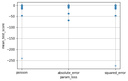
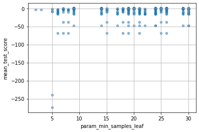
以下の図を見ればわかりますが、最初の iteration の RandomSearchCV で決めたパラメータを変更することなく resource だけ変更しているようです。ここんとこ、改善の余地がありそうな気がしますね。

for col in cv_results_df.columns:
    if col[:6] == "param_":
        cv_results_df.plot(col, "mean_test_score", kind="scatter", alpha=0.5, grid=True)

おわりに

というわけで、scikit-learn の GridSearchCV とその兄弟たち HalvingGridSearchCV RandomizedSearchCV HalvingRandomSearchCV を使ってみました。その挙動は色々と参考になりますが、個人的にはやっぱりOptunaが柔軟な使い方ができて良いかなと再認識しました。私が使いこなしてないだけかもしれませんが。

You get articles that match your needs
You can efficiently read back useful information
You can use dark theme

What you can do with signing up