最適なパラメータを効率的に探索しちゃおっちゅうな(Optuna)

グリッドサーチよりも良いと言われるハイパーパラメータ探索手法 Optuna を私も試しちゃおっちゅうな話です。以下のコードは全て Google Colaboratory 上で動かしましたっちゅうなことです。

Optuna のインストール

Google Colaboratory 上に Optuna はなかったので pip install しました。簡単。

!pip install optuna

Collecting optuna
[?25l  Downloading https://files.pythonhosted.org/packages/d4/6a/4d80b3014797cf318a5252afb27031e9e7502854fb7930f27db0ee10bb75/optuna-0.19.0.tar.gz (126kB)
[K     |████████████████████████████████| 133kB 4.9MB/s 
[?25hCollecting alembic
[?25l  Downloading https://files.pythonhosted.org/packages/84/64/493c45119dce700a4b9eeecc436ef9e8835ab67bae6414f040cdc7b58f4b/alembic-1.3.1.tar.gz (1.1MB)
[K     |████████████████████████████████| 1.1MB 42.4MB/s 
[?25hCollecting cliff
[?25l  Downloading https://files.pythonhosted.org/packages/f6/a9/e976ba91e57043c4b6add2c394e6d1ffc26712c694379c3fe72f942d2440/cliff-2.16.0-py2.py3-none-any.whl (78kB)
[K     |████████████████████████████████| 81kB 8.5MB/s 
[?25hCollecting colorlog
  Downloading https://files.pythonhosted.org/packages/68/4d/892728b0c14547224f0ac40884e722a3d00cb54e7a146aea0b3186806c9e/colorlog-4.0.2-py2.py3-none-any.whl
Requirement already satisfied: numpy in /usr/local/lib/python3.6/dist-packages (from optuna) (1.17.4)
Requirement already satisfied: scipy in /usr/local/lib/python3.6/dist-packages (from optuna) (1.3.3)
Requirement already satisfied: six in /usr/local/lib/python3.6/dist-packages (from optuna) (1.12.0)
Requirement already satisfied: sqlalchemy>=1.1.0 in /usr/local/lib/python3.6/dist-packages (from optuna) (1.3.11)
Requirement already satisfied: tqdm in /usr/local/lib/python3.6/dist-packages (from optuna) (4.28.1)
Requirement already satisfied: typing in /usr/local/lib/python3.6/dist-packages (from optuna) (3.6.6)
Collecting Mako
[?25l  Downloading https://files.pythonhosted.org/packages/b0/3c/8dcd6883d009f7cae0f3157fb53e9afb05a0d3d33b3db1268ec2e6f4a56b/Mako-1.1.0.tar.gz (463kB)
[K     |████████████████████████████████| 471kB 37.3MB/s 
[?25hCollecting python-editor>=0.3
  Downloading https://files.pythonhosted.org/packages/c6/d3/201fc3abe391bbae6606e6f1d598c15d367033332bd54352b12f35513717/python_editor-1.0.4-py3-none-any.whl
Requirement already satisfied: python-dateutil in /usr/local/lib/python3.6/dist-packages (from alembic->optuna) (2.6.1)
Requirement already satisfied: PyYAML>=3.12 in /usr/local/lib/python3.6/dist-packages (from cliff->optuna) (3.13)
Collecting cmd2!=0.8.3,<0.9.0,>=0.8.0
[?25l  Downloading https://files.pythonhosted.org/packages/e9/40/a71caa2aaff10c73612a7106e2d35f693e85b8cf6e37ab0774274bca3cf9/cmd2-0.8.9-py2.py3-none-any.whl (53kB)
[K     |████████████████████████████████| 61kB 7.7MB/s 
[?25hCollecting pbr!=2.1.0,>=2.0.0
[?25l  Downloading https://files.pythonhosted.org/packages/7a/db/a968fd7beb9fe06901c1841cb25c9ccb666ca1b9a19b114d1bbedf1126fc/pbr-5.4.4-py2.py3-none-any.whl (110kB)
[K     |████████████████████████████████| 112kB 36.3MB/s 
[?25hRequirement already satisfied: pyparsing>=2.1.0 in /usr/local/lib/python3.6/dist-packages (from cliff->optuna) (2.4.5)
Collecting stevedore>=1.20.0
[?25l  Downloading https://files.pythonhosted.org/packages/b1/e1/f5ddbd83f60b03f522f173c03e406c1bff8343f0232a292ac96aa633b47a/stevedore-1.31.0-py2.py3-none-any.whl (43kB)
[K     |████████████████████████████████| 51kB 6.5MB/s 
[?25hRequirement already satisfied: PrettyTable<0.8,>=0.7.2 in /usr/local/lib/python3.6/dist-packages (from cliff->optuna) (0.7.2)
Requirement already satisfied: MarkupSafe>=0.9.2 in /usr/local/lib/python3.6/dist-packages (from Mako->alembic->optuna) (1.1.1)
Requirement already satisfied: wcwidth; sys_platform != "win32" in /usr/local/lib/python3.6/dist-packages (from cmd2!=0.8.3,<0.9.0,>=0.8.0->cliff->optuna) (0.1.7)
Collecting pyperclip
  Downloading https://files.pythonhosted.org/packages/2d/0f/4eda562dffd085945d57c2d9a5da745cfb5228c02bc90f2c74bbac746243/pyperclip-1.7.0.tar.gz
Building wheels for collected packages: optuna, alembic, Mako, pyperclip
  Building wheel for optuna (setup.py) ... [?25l[?25hdone
  Created wheel for optuna: filename=optuna-0.19.0-cp36-none-any.whl size=170198 sha256=fdc7777d7454f3419bc9acfd4f83f5cf6f23f0d6a6f392fc744afb597484f156
  Stored in directory: /root/.cache/pip/wheels/49/bf/47/090a43457caeff74397397da1c98a8aaed685257c16a5ba1f0
  Building wheel for alembic (setup.py) ... [?25l[?25hdone
  Created wheel for alembic: filename=alembic-1.3.1-py2.py3-none-any.whl size=144523 sha256=c66d5c3c4bd291757c2136352ac8d3cab450cccd0cb1005fe01211c5fa7576f4
  Stored in directory: /root/.cache/pip/wheels/b2/d4/19/5ab879d30af7cbc79e6dcc1d421795b1aa9d78f455b0412ef7
  Building wheel for Mako (setup.py) ... [?25l[?25hdone
  Created wheel for Mako: filename=Mako-1.1.0-cp36-none-any.whl size=75363 sha256=66ee5267f833ecdf52af2f6c7e8c93bb317a780d609f0765a8101383516ab29b
  Stored in directory: /root/.cache/pip/wheels/98/32/7b/a291926643fc1d1e02593e0d9e247c5a866a366b8343b7aa27
  Building wheel for pyperclip (setup.py) ... [?25l[?25hdone
  Created wheel for pyperclip: filename=pyperclip-1.7.0-cp36-none-any.whl size=8359 sha256=7e62cb6b9e2dcb8a323251caa96de1064b10e0a80baaf6b33b2052fafa34c08e
  Stored in directory: /root/.cache/pip/wheels/92/f0/ac/2ba2972034e98971c3654ece337ac61e546bdeb34ca960dc8c
Successfully built optuna alembic Mako pyperclip
Installing collected packages: Mako, python-editor, alembic, pyperclip, cmd2, pbr, stevedore, cliff, colorlog, optuna
Successfully installed Mako-1.1.0 alembic-1.3.1 cliff-2.16.0 cmd2-0.8.9 colorlog-4.0.2 optuna-0.19.0 pbr-5.4.4 pyperclip-1.7.0 python-editor-1.0.4 stevedore-1.31.0

インストールがうまくいったようなので、次の import 文を命令して、動作確認。

import optuna

準備体操

まずは Optuna の動作を理解するための準備体操から。

１変数の関数の最小化

試しに $f(x) = x^4 - 4x^3 - 36x^2$ を最小化してみます。

def f(x):
    return x**4 - 4 * x ** 3 - 36 * x ** 2

Optunaでは、最小化したい目的関数は次のように定義します。

def objective(trial):
    x = trial.suggest_uniform('x', -10, 10)
    return f(x)

次のようにすれば、10回だけ試行してくれます。

study = optuna.create_study()
study.optimize(objective, n_trials=10)

[32m[I 2019-12-13 00:32:08,911][0m Finished trial#0 resulted in value: 2030.566599827237. Current best value is 2030.566599827237 with parameters: {'x': 9.815207070259166}.[0m
[32m[I 2019-12-13 00:32:09,021][0m Finished trial#1 resulted in value: 1252.1813135138896. Current best value is 1252.1813135138896 with parameters: {'x': 9.366926766768199}.[0m
[32m[I 2019-12-13 00:32:09,147][0m Finished trial#2 resulted in value: -283.8813965725701. Current best value is -283.8813965725701 with parameters: {'x': 2.6795376432294855}.[0m
[32m[I 2019-12-13 00:32:09,278][0m Finished trial#3 resulted in value: 1258.1505983061907. Current best value is -283.8813965725701 with parameters: {'x': 2.6795376432294855}.[0m
[32m[I 2019-12-13 00:32:09,409][0m Finished trial#4 resulted in value: -59.988164166655146. Current best value is -283.8813965725701 with parameters: {'x': 2.6795376432294855}.[0m
[32m[I 2019-12-13 00:32:09,539][0m Finished trial#5 resulted in value: 6493.216295606622. Current best value is -283.8813965725701 with parameters: {'x': 2.6795376432294855}.[0m
[32m[I 2019-12-13 00:32:09,670][0m Finished trial#6 resulted in value: 233.47766027651414. Current best value is -283.8813965725701 with parameters: {'x': 2.6795376432294855}.[0m
[32m[I 2019-12-13 00:32:09,797][0m Finished trial#7 resulted in value: -32.56782816991587. Current best value is -283.8813965725701 with parameters: {'x': 2.6795376432294855}.[0m
[32m[I 2019-12-13 00:32:09,924][0m Finished trial#8 resulted in value: 9713.778056852296. Current best value is -283.8813965725701 with parameters: {'x': 2.6795376432294855}.[0m
[32m[I 2019-12-13 00:32:10,046][0m Finished trial#9 resulted in value: -499.577141711988. Current best value is -499.577141711988 with parameters: {'x': 3.6629193285453887}.[0m

試行回数を確認すると

len(study.trials)

10

目的関数を最小化するパラメータは次のようにして確認できます。

study.best_params

{'x': 3.6629193285453887}

目的関数の最小値は次のようにして得られます。

study.best_value

-499.577141711988

最小値を得た試行の情報はこのようにして得られます。

study.best_trial

FrozenTrial(number=9, state=TrialState.COMPLETE, value=-499.577141711988, datetime_start=datetime.datetime(2019, 12, 13, 0, 32, 9, 926514), datetime_complete=datetime.datetime(2019, 12, 13, 0, 32, 10, 46429), params={'x': 3.6629193285453887}, distributions={'x': UniformDistribution(high=10, low=-10)}, user_attrs={}, system_attrs={'_number': 9}, intermediate_values={}, trial_id=9)

試行の履歴はこのようにして見られます。

study.trials

[FrozenTrial(number=0, state=TrialState.COMPLETE, value=2030.566599827237, datetime_start=datetime.datetime(2019, 12, 13, 0, 32, 8, 821843), datetime_complete=datetime.datetime(2019, 12, 13, 0, 32, 8, 911548), params={'x': 9.815207070259166}, distributions={'x': UniformDistribution(high=10, low=-10)}, user_attrs={}, system_attrs={'_number': 0}, intermediate_values={}, trial_id=0),
 FrozenTrial(number=1, state=TrialState.COMPLETE, value=1252.1813135138896, datetime_start=datetime.datetime(2019, 12, 13, 0, 32, 8, 912983), datetime_complete=datetime.datetime(2019, 12, 13, 0, 32, 9, 20790), params={'x': 9.366926766768199}, distributions={'x': UniformDistribution(high=10, low=-10)}, user_attrs={}, system_attrs={'_number': 1}, intermediate_values={}, trial_id=1),
 FrozenTrial(number=2, state=TrialState.COMPLETE, value=-283.8813965725701, datetime_start=datetime.datetime(2019, 12, 13, 0, 32, 9, 22532), datetime_complete=datetime.datetime(2019, 12, 13, 0, 32, 9, 147430), params={'x': 2.6795376432294855}, distributions={'x': UniformDistribution(high=10, low=-10)}, user_attrs={}, system_attrs={'_number': 2}, intermediate_values={}, trial_id=2),
 FrozenTrial(number=3, state=TrialState.COMPLETE, value=1258.1505983061907, datetime_start=datetime.datetime(2019, 12, 13, 0, 32, 9, 149953), datetime_complete=datetime.datetime(2019, 12, 13, 0, 32, 9, 277900), params={'x': 9.37074944280344}, distributions={'x': UniformDistribution(high=10, low=-10)}, user_attrs={}, system_attrs={'_number': 3}, intermediate_values={}, trial_id=3),
 FrozenTrial(number=4, state=TrialState.COMPLETE, value=-59.988164166655146, datetime_start=datetime.datetime(2019, 12, 13, 0, 32, 9, 281543), datetime_complete=datetime.datetime(2019, 12, 13, 0, 32, 9, 409038), params={'x': -1.4636181925092284}, distributions={'x': UniformDistribution(high=10, low=-10)}, user_attrs={}, system_attrs={'_number': 4}, intermediate_values={}, trial_id=4),
 FrozenTrial(number=5, state=TrialState.COMPLETE, value=6493.216295606622, datetime_start=datetime.datetime(2019, 12, 13, 0, 32, 9, 410813), datetime_complete=datetime.datetime(2019, 12, 13, 0, 32, 9, 539381), params={'x': -8.979003291609324}, distributions={'x': UniformDistribution(high=10, low=-10)}, user_attrs={}, system_attrs={'_number': 5}, intermediate_values={}, trial_id=5),
 FrozenTrial(number=6, state=TrialState.COMPLETE, value=233.47766027651414, datetime_start=datetime.datetime(2019, 12, 13, 0, 32, 9, 542239), datetime_complete=datetime.datetime(2019, 12, 13, 0, 32, 9, 669699), params={'x': -5.01912242330347}, distributions={'x': UniformDistribution(high=10, low=-10)}, user_attrs={}, system_attrs={'_number': 6}, intermediate_values={}, trial_id=6),
 FrozenTrial(number=7, state=TrialState.COMPLETE, value=-32.56782816991587, datetime_start=datetime.datetime(2019, 12, 13, 0, 32, 9, 671679), datetime_complete=datetime.datetime(2019, 12, 13, 0, 32, 9, 797441), params={'x': -1.027752432268013}, distributions={'x': UniformDistribution(high=10, low=-10)}, user_attrs={}, system_attrs={'_number': 7}, intermediate_values={}, trial_id=7),
 FrozenTrial(number=8, state=TrialState.COMPLETE, value=9713.778056852296, datetime_start=datetime.datetime(2019, 12, 13, 0, 32, 9, 799124), datetime_complete=datetime.datetime(2019, 12, 13, 0, 32, 9, 924648), params={'x': -9.843104909274034}, distributions={'x': UniformDistribution(high=10, low=-10)}, user_attrs={}, system_attrs={'_number': 8}, intermediate_values={}, trial_id=8),
 FrozenTrial(number=9, state=TrialState.COMPLETE, value=-499.577141711988, datetime_start=datetime.datetime(2019, 12, 13, 0, 32, 9, 926514), datetime_complete=datetime.datetime(2019, 12, 13, 0, 32, 10, 46429), params={'x': 3.6629193285453887}, distributions={'x': UniformDistribution(high=10, low=-10)}, user_attrs={}, system_attrs={'_number': 9}, intermediate_values={}, trial_id=9)]

では、追加で１００回試行してみましょう。

study.optimize(objective, n_trials=100)

[32m[I 2019-12-13 00:32:10,303][0m Finished trial#10 resulted in value: -679.8303609251094. Current best value is -679.8303609251094 with parameters: {'x': 4.482235669344949}.[0m
[32m[I 2019-12-13 00:32:10,447][0m Finished trial#11 resulted in value: -664.7000624843927. Current best value is -679.8303609251094 with parameters: {'x': 4.482235669344949}.[0m
[32m[I 2019-12-13 00:32:10,579][0m Finished trial#12 resulted in value: -778.9261500173968. Current best value is -778.9261500173968 with parameters: {'x': 5.024746639127292}.[0m
...（中略）...
[32m[I 2019-12-13 00:32:22,591][0m Finished trial#107 resulted in value: -760.7787838740135. Current best value is -863.9855798856751 with parameters: {'x': 6.011542730094907}.[0m
[32m[I 2019-12-13 00:32:22,724][0m Finished trial#108 resulted in value: -773.0113811629133. Current best value is -863.9855798856751 with parameters: {'x': 6.011542730094907}.[0m
[32m[I 2019-12-13 00:32:22,862][0m Finished trial#109 resulted in value: -577.7178004902428. Current best value is -863.9855798856751 with parameters: {'x': 6.011542730094907}.[0m

これで、試行回数は

len(study.trials)

110

目的関数を最小化するパラメータと、そのときの目的関数の値は

study.best_params, study.best_value

({'x': 6.011542730094907}, -863.9855798856751)

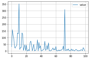
目的関数の値の履歴は次のように可視化できます。

%matplotlib inline
import matplotlib.pyplot as plt

plt.plot([trial.value for trial in study.trials])
plt.grid()
plt.show()

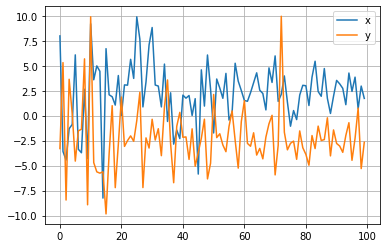
パラメータの履歴は次のように可視化できます。

%matplotlib inline
import matplotlib.pyplot as plt

plt.plot([trial.params['x'] for trial in study.trials])
plt.grid()
plt.show()

パラメータの探索がどのように行われたのか図示してみましょう。

%matplotlib inline
import matplotlib.pyplot as plt

plt.grid()
plt.plot([trial.params['x'] for trial in study.trials], 
         [trial.value for trial in study.trials],
         marker='x', alpha=0.3)
plt.scatter(study.trials[0].params['x'], study.trials[0].value, 
         marker='>', label='start', s=100)
plt.scatter(study.trials[-1].params['x'], study.trials[-1].value, 
         marker='s', label='end', s=100)
plt.scatter(study.best_params['x'], study.best_value,
         marker='o', label='best', s=100)
plt.xlabel('x')
plt.ylabel('y (value)')
plt.legend()
plt.show()

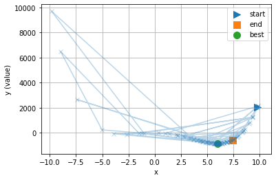
最小値が期待できなさそうな領域はそこそこにして、期待できそうな領域を重点的に探索したことが分かります。

２変数の関数の最小化

次は $f(x, y) = (x - 2.5)^2 + 2 (y + 2.5) ^ 2$ を最小化してみましょう。

def f(x, y):
    return (x - 2.5)**2 + 2 * (y + 2.5) ** 2

最小化したい関数の定義

def objective(trial):
    x = trial.suggest_uniform('x', -10, 10)
    y = trial.suggest_uniform('y', -10, 10)
    return f(x, y)

こうして100回試行して

study = optuna.create_study()
study.optimize(objective, n_trials=100)

[32m[I 2019-12-13 00:32:24,001][0m Finished trial#0 resulted in value: 31.229461850588567. Current best value is 31.229461850588567 with parameters: {'x': 7.975371679174145, 'y': -3.290495675347522}.[0m
[32m[I 2019-12-13 00:32:24,131][0m Finished trial#1 resulted in value: 158.84900024337801. Current best value is 31.229461850588567 with parameters: {'x': 7.975371679174145, 'y': -3.290495675347522}.[0m
[32m[I 2019-12-13 00:32:24,252][0m Finished trial#2 resulted in value: 118.67648241872055. Current best value is 31.229461850588567 with parameters: {'x': 7.975371679174145, 'y': -3.290495675347522}.[0m
...（中略）...
[32m[I 2019-12-13 00:32:37,321][0m Finished trial#97 resulted in value: 24.46020780084274. Current best value is 0.2114497716311141 with parameters: {'x': 2.286816304129357, 'y': -2.788099360851467}.[0m
[32m[I 2019-12-13 00:32:37,471][0m Finished trial#98 resulted in value: 15.832787347997524. Current best value is 0.2114497716311141 with parameters: {'x': 2.286816304129357, 'y': -2.788099360851467}.[0m
[32m[I 2019-12-13 00:32:37,625][0m Finished trial#99 resulted in value: 0.6493005675217599. Current best value is 0.2114497716311141 with parameters: {'x': 2.286816304129357, 'y': -2.788099360851467}.[0m

目的関数を最小化するパラメータと、そのときの最小値

study.best_params, study.best_value

({'x': 2.286816304129357, 'y': -2.788099360851467}, 0.2114497716311141)

目的関数の値とパラメータの履歴

%matplotlib inline
import matplotlib.pyplot as plt

plt.plot([trial.value for trial in study.trials], label='value')
plt.grid()
plt.legend()
plt.show()

plt.plot([trial.params['x'] for trial in study.trials], label='x')
plt.plot([trial.params['y'] for trial in study.trials], label='y')
plt.grid()
plt.legend()
plt.show()

パラメータの履歴を二次元平面上に図示してみましょう。

%matplotlib inline
import matplotlib.pyplot as plt

plt.plot([trial.params['x'] for trial in study.trials], 
         [trial.params['y'] for trial in study.trials],
         alpha=0.4, marker='x')
plt.scatter(study.trials[0].params['x'], study.trials[0].params['y'], 
         marker='>', label='start', s=100)
plt.scatter(study.trials[-1].params['x'], study.trials[-1].params['y'], 
         marker='s', label='end', s=100)
plt.scatter(study.best_params['x'], study.best_params['y'],
         marker='o', label='best', s=100)
plt.grid()
plt.legend()
plt.show()

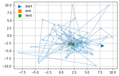
ここでも、最小値が期待できなさそうな領域はそこそこにして、期待できそうな領域を重点的に探索したことが分かります。

以上、Optunaの動作を簡単に把握するための準備体操でした。

教師あり機械学習への応用

ここから、これを教師あり機械学習のハイパーパラメーターチューニングに応用します。

乳がんデータセット

機械学習ライブラリ Scikit-learn の breast cancer datasets を例に用い、説明変数 $X$ と目的変数 $y$ を次のように得ます。

# https://scikit-learn.org/stable/modules/generated/sklearn.datasets.load_breast_cancer.html
from sklearn.datasets import load_breast_cancer
breast_cancer = load_breast_cancer()
X = breast_cancer.data
y = breast_cancer.target.ravel()

訓練データとテストデータに分割します。

from sklearn.model_selection import train_test_split 
# 訓練データ・テストデータへ6:4の比でランダムに分割
X_train, X_test, y_train, y_test = train_test_split(X, y, test_size=.4) 

比較対象としてのグリッドサーチ

Optuna との比較として、グリッドサーチの復習をします。グリッドサーチでは、与えられた「パラメータの値の候補」の全組み合わせを試行し、その中から性能が最も良いものを選びます。教師あり機械学習の例として lightGBM を使うと、こんな感じです。

%%time
from sklearn.model_selection import GridSearchCV

# LightGBM
import lightgbm as lgb

# グリッドサーチを行うためのパラメーター
parameters = [{
    'learning_rate':[0.1,0.2],
    'n_estimators':[20,100,200],
    'max_depth':[3,5,7,9],
    'min_child_weight':[0.5,1,2],
    'min_child_samples':[5,10,20],
    'subsample':[0.8],
    'colsample_bytree':[0.8],
    'verbose':[-1],
    'num_leaves':[80]
}]

#グリッドサーチ実行
classifier = GridSearchCV(lgb.LGBMClassifier(), parameters, cv=3, n_jobs=-1)
classifier.fit(X_train, y_train)
print("Accuracy score (train): ", classifier.score(X_train, y_train))
print("Accuracy score (test): ", classifier.score(X_test, y_test))
print(classifier.best_estimator_) # ベストのパラメーター

Accuracy score (train):  1.0
Accuracy score (test):  0.9517543859649122
LGBMClassifier(boosting_type='gbdt', class_weight=None, colsample_bytree=0.8,
               importance_type='split', learning_rate=0.1, max_depth=3,
               min_child_samples=20, min_child_weight=0.5, min_split_gain=0.0,
               n_estimators=100, n_jobs=-1, num_leaves=80, objective=None,
               random_state=None, reg_alpha=0.0, reg_lambda=0.0, silent=True,
               subsample=0.8, subsample_for_bin=200000, subsample_freq=0,
               verbose=-1)
CPU times: user 1.15 s, sys: 109 ms, total: 1.26 s
Wall time: 15.3 s

グリッドサーチの特徴は

• あらかじめ与えられた値のみを使う。
• 全組み合わせを試す。

で、期待できるところを重点的に探索、などはしません。

LightGBM + Optuna

では、このLightGBMをグリッドサーチではなくOptunaでチューニングしてみましょう。

import numpy as np
# 目的関数
def objective(trial):
    learning_rate = trial.suggest_loguniform('learning_rate', 0.1,0.2),
    n_estimators, = trial.suggest_int('n_estimators', 20, 200),
    max_depth, = trial.suggest_int('max_depth', 3, 9),
    min_child_weight = trial.suggest_loguniform('min_child_weight', 0.5, 2),
    min_child_samples, = trial.suggest_int('min_child_samples', 5, 20),
    classifier = lgb.LGBMClassifier(learning_rate=learning_rate, 
                                    n_estimators=n_estimators,
                                    max_depth=max_depth, 
                                    min_child_weight=min_child_weight,
                                    min_child_samples=min_child_samples,
                                    subsample=0.8, colsample_bytree=0.8,
                                    verbose=-1, num_leaves=80)
    classifier.fit(X_train, y_train)
    #return classifier.score(X_train, y_train) # 正答率（train） の最適化
    return np.linalg.norm(y_train - classifier.predict_proba(X_train)[:, 1], ord=1) # 尤度の最適化

上の関数で、何を最適化すればよいかは選択の余地があると思います。用いた lightGBMは「回帰」ではなく「分類」をする学習器で、

classifier.score(X_train, y_train) を用いると、正答率（train） を最適化することになります。分類における正答率は、何個のデータ中何個が正しく分類されたかという数字ですので、連続値に見えて、実質、離散値に近い数字です。例えば、１０個中８個が正しく分類されたとして、その分類が「余裕の正解」だろうと「ギリギリ正解」だろうと正答率（train）は変わりません。つまり、「ギリギリ正解」から「余裕の正解」に近づける力が働きにくいのです。

np.linalg.norm(y_train - classifier.predict_proba(X_train)[:, 1], ord=1) を用いると、これが回避できます。この中の y_train は、分類結果が0か1かという教師セット、classifier.predict_proba(X_train)[:, 1] は、予測が1であるという自身の強さ（確率に相当するもの）です。この２つの値の差の L1ノルム （L2ノルムでも構わないと思います）を最小化することで、「不正解」を「正解」に、「ギリギリ正解」から「余裕の正解」に近づける力を働きやすくします。

では、学習を開始しましょう。もし classifier.score(X_train, y_train) を用いた場合はその最大化を選びます。もし np.linalg.norm(y_train - classifier.predict_proba(X_train)[:, 1], ord=1) を用いた場合はその最小化を選びます。

#study = optuna.create_study(direction='maximize') # 最大化
study = optuna.create_study(direction='minimize') # 最小化

こうして100回試行して

study.optimize(objective, n_trials=100)

[32m[I 2019-12-13 00:32:54,913][0m Finished trial#0 resulted in value: 1.5655193925176527. Current best value is 1.5655193925176527 with parameters: {'learning_rate': 0.11563458547060446, 'n_estimators': 155, 'max_depth': 7, 'min_child_weight': 0.7324812463494225, 'min_child_samples': 12}.[0m
[32m[I 2019-12-13 00:32:55,103][0m Finished trial#1 resulted in value: 1.3810988452320123. Current best value is 1.3810988452320123 with parameters: {'learning_rate': 0.15351688726053717, 'n_estimators': 83, 'max_depth': 6, 'min_child_weight': 0.5802652538400225, 'min_child_samples': 8}.[0m
[32m[I 2019-12-13 00:32:55,287][0m Finished trial#2 resulted in value: 3.519787362063691. Current best value is 1.3810988452320123 with parameters: {'learning_rate': 0.15351688726053717, 'n_estimators': 83, 'max_depth': 6, 'min_child_weight': 0.5802652538400225, 'min_child_samples': 8}.[0m
...（中略）...
[32m[I 2019-12-13 00:33:17,608][0m Finished trial#97 resulted in value: 1.0443245090791662. Current best value is 1.0230542364962214 with parameters: {'learning_rate': 0.11851649444429455, 'n_estimators': 176, 'max_depth': 9, 'min_child_weight': 0.50006741615294, 'min_child_samples': 8}.[0m
[32m[I 2019-12-13 00:33:17,871][0m Finished trial#98 resulted in value: 1.3997762969822483. Current best value is 1.0230542364962214 with parameters: {'learning_rate': 0.11851649444429455, 'n_estimators': 176, 'max_depth': 9, 'min_child_weight': 0.50006741615294, 'min_child_samples': 8}.[0m
[32m[I 2019-12-13 00:33:18,187][0m Finished trial#99 resulted in value: 1.1059309199723422. Current best value is 1.0230542364962214 with parameters: {'learning_rate': 0.11851649444429455, 'n_estimators': 176, 'max_depth': 9, 'min_child_weight': 0.50006741615294, 'min_child_samples': 8}.[0m

目的関数を最適化するパラメーターは

study.best_params

{'learning_rate': 0.11851649444429455,
 'max_depth': 9,
 'min_child_samples': 8,
 'min_child_weight': 0.50006741615294,
 'n_estimators': 176}

こんなキリの悪そうな値を、グリッドサーチでは、求められそうにないですね。

そしてそのときの最適値は

study.best_value

1.0230542364962214

得られた最適パラメータは、**study.best_params を用いて代入して、チューニング後の分類器を作れます。

classifier = lgb.LGBMClassifier(**study.best_params,
                                subsample=0.8, colsample_bytree=0.8,
                                verbose=-1, num_leaves=80)
classifier

LGBMClassifier(boosting_type='gbdt', class_weight=None, colsample_bytree=0.8,
               importance_type='split', learning_rate=0.11851649444429455,
               max_depth=9, min_child_samples=8,
               min_child_weight=0.50006741615294, min_split_gain=0.0,
               n_estimators=176, n_jobs=-1, num_leaves=80, objective=None,
               random_state=None, reg_alpha=0.0, reg_lambda=0.0, silent=True,
               subsample=0.8, subsample_for_bin=200000, subsample_freq=0,
               verbose=-1)

ベストな分類器で学習

classifier.fit(X_train, y_train)

LGBMClassifier(boosting_type='gbdt', class_weight=None, colsample_bytree=0.8,
               importance_type='split', learning_rate=0.11851649444429455,
               max_depth=9, min_child_samples=8,
               min_child_weight=0.50006741615294, min_split_gain=0.0,
               n_estimators=176, n_jobs=-1, num_leaves=80, objective=None,
               random_state=None, reg_alpha=0.0, reg_lambda=0.0, silent=True,
               subsample=0.8, subsample_for_bin=200000, subsample_freq=0,
               verbose=-1)

そして予測

classifier.score(X_train, y_train)

1.0

classifier.score(X_test, y_test)

0.9473684210526315

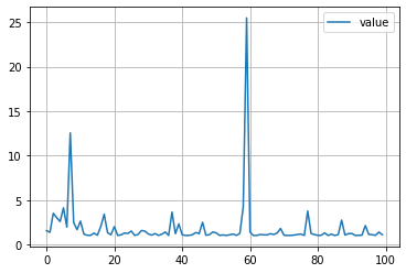
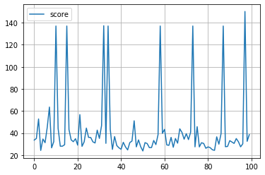
目的関数の値の履歴

plt.plot([trial.value for trial in study.trials], label='value')
plt.grid()
plt.legend()
plt.show()

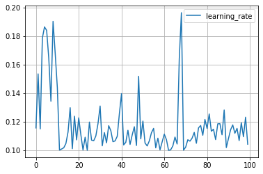
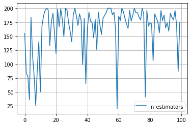
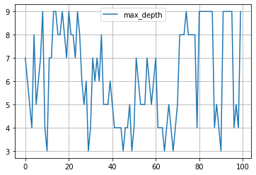
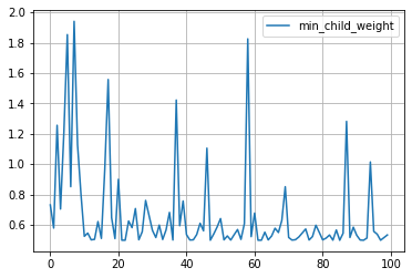
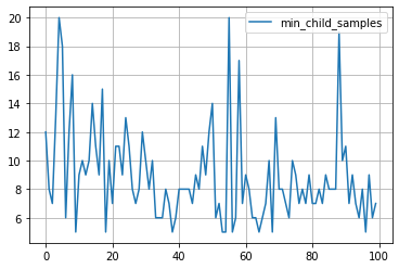
パラメータ探索の履歴

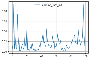
for key in study.trials[0].params.keys():
    plt.plot([trial.params[key] for trial in study.trials], label=key)
    plt.grid()
    plt.legend()
    plt.show()

という具合です。

scikit-learn/MLP + Optuna

同様に、scikit-learnの多層パーセプトロンをチューニングしてみましょう。まずはグリッドサーチから。

%%time
from sklearn.model_selection import GridSearchCV

# 多層パーセプトロン
from sklearn.neural_network import MLPClassifier
# グリッドサーチを行うためのパラメーター
parameters = [{'hidden_layer_sizes': [8, 16, 32, (8, 8), (8, 8, 8)], 
               'solver': ['adam'], 'activation': ['relu'],
              'learning_rate_init': [0.1, 0.01, 0.001]}]
#グリッドサーチ実行
classifier = GridSearchCV(MLPClassifier(max_iter=10000, early_stopping=True), 
                          parameters, cv=3, n_jobs=-1)
classifier.fit(X_train, y_train)
print("Accuracy score (train): ", classifier.score(X_train, y_train))
print("Accuracy score (test): ", classifier.score(X_test, y_test))
print(classifier.best_estimator_) # ベストのパラメーターを持つ分類器

Accuracy score (train):  0.9090909090909091
Accuracy score (test):  0.8728070175438597
MLPClassifier(activation='relu', alpha=0.0001, batch_size='auto', beta_1=0.9,
              beta_2=0.999, early_stopping=True, epsilon=1e-08,
              hidden_layer_sizes=32, learning_rate='constant',
              learning_rate_init=0.1, max_iter=10000, momentum=0.9,
              n_iter_no_change=10, nesterovs_momentum=True, power_t=0.5,
              random_state=None, shuffle=True, solver='adam', tol=0.0001,
              validation_fraction=0.1, verbose=False, warm_start=False)
CPU times: user 166 ms, sys: 30.3 ms, total: 196 ms
Wall time: 3.07 s

多層パーセプトロンでは、

• 隠れ層を何層にするか
• それぞれの層のサイズをどのくらいにするか

というファクターがあるので、ちょっと大変です。

隠れ層を１層に固定

# 目的関数
def objective(trial):
    hidden_layer_sizes, = trial.suggest_int('hidden_layer_sizes', 8, 100),
    learning_rate_init, = trial.suggest_loguniform('learning_rate_init', 0.001, 0.1),
    classifier = MLPClassifier(max_iter=10000, early_stopping=True,
                                    hidden_layer_sizes=hidden_layer_sizes,
                                    learning_rate_init=learning_rate_init, 
                                    solver='adam', activation='relu')
    classifier.fit(X_train, y_train)
    #return classifier.score(X_train, y_train)
    #return classifier.score(X_test, y_test)
    return np.linalg.norm(y_train - classifier.predict_proba(X_train)[:, 1], ord=1)

#study = optuna.create_study(direction='maximize')
study = optuna.create_study(direction='minimize')
study.optimize(objective, n_trials=100)

[32m[I 2019-12-13 00:33:23,314][0m Finished trial#0 resulted in value: 33.67375867333378. Current best value is 33.67375867333378 with parameters: {'hidden_layer_sizes': 73, 'learning_rate_init': 0.004548472515805296}.[0m
[32m[I 2019-12-13 00:33:23,538][0m Finished trial#1 resulted in value: 35.17385235930611. Current best value is 33.67375867333378 with parameters: {'hidden_layer_sizes': 73, 'learning_rate_init': 0.004548472515805296}.[0m
[32m[I 2019-12-13 00:33:23,716][0m Finished trial#2 resulted in value: 52.815452458627675. Current best value is 33.67375867333378 with parameters: {'hidden_layer_sizes': 73, 'learning_rate_init': 0.004548472515805296}.[0m
...（中略）...
[32m[I 2019-12-13 00:33:47,631][0m Finished trial#97 resulted in value: 150.15953891394736. Current best value is 23.844866313445344 with parameters: {'hidden_layer_sizes': 79, 'learning_rate_init': 0.010242027297662661}.[0m
[32m[I 2019-12-13 00:33:47,894][0m Finished trial#98 resulted in value: 32.56506872305802. Current best value is 23.844866313445344 with parameters: {'hidden_layer_sizes': 79, 'learning_rate_init': 0.010242027297662661}.[0m
[32m[I 2019-12-13 00:33:48,172][0m Finished trial#99 resulted in value: 38.57363524502563. Current best value is 23.844866313445344 with parameters: {'hidden_layer_sizes': 79, 'learning_rate_init': 0.010242027297662661}.[0m

study.best_params

{'hidden_layer_sizes': 79, 'learning_rate_init': 0.010242027297662661}

study.best_value

23.844866313445344

classifier = MLPClassifier(**study.best_params)
classifier.fit(X_train, y_train)
classifier.score(X_train, y_train), classifier.score(X_test, y_test)

(0.9472140762463344, 0.9122807017543859)

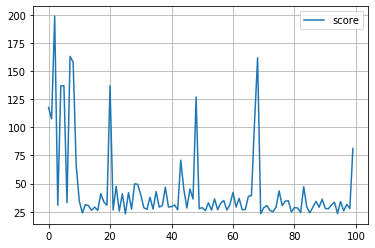
plt.plot([trial.value for trial in study.trials], label='score')
plt.grid()
plt.legend()
plt.show()

for key in study.trials[0].params.keys():
    plt.plot([trial.params[key] for trial in study.trials], label=key)
    plt.grid()
    plt.legend()
    plt.show()

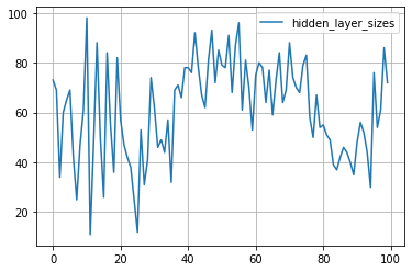
隠れ層を2層に固定

# 目的関数
def objective(trial):
    h1, = trial.suggest_int('h1', 8, 100),
    h2, = trial.suggest_int('h2', 8, 100),
    learning_rate_init, = trial.suggest_loguniform('learning_rate_init', 0.001, 0.1),
    classifier = MLPClassifier(max_iter=10000, early_stopping=True,
                                    hidden_layer_sizes=(h1, h2),
                                    learning_rate_init=learning_rate_init, 
                                    solver='adam', activation='relu')
    classifier.fit(X_train, y_train)
    #return classifier.score(X_train, y_train)
    #return classifier.score(X_test, y_test)
    return np.linalg.norm(y_train - classifier.predict_proba(X_train)[:, 1], ord=1)

#study = optuna.create_study(direction='maximize')
study = optuna.create_study(direction='minimize')
study.optimize(objective, n_trials=100)

[32m[I 2019-12-13 00:33:49,555][0m Finished trial#0 resulted in value: 44.26353774856942. Current best value is 44.26353774856942 with parameters: {'h1': 15, 'h2': 99, 'learning_rate_init': 0.003018305556292618}.[0m
[32m[I 2019-12-13 00:33:49,851][0m Finished trial#1 resulted in value: 29.450960862380153. Current best value is 29.450960862380153 with parameters: {'h1': 81, 'h2': 79, 'learning_rate_init': 0.01344672244443261}.[0m
[32m[I 2019-12-13 00:33:50,073][0m Finished trial#2 resulted in value: 38.96850500173973. Current best value is 29.450960862380153 with parameters: {'h1': 81, 'h2': 79, 'learning_rate_init': 0.01344672244443261}.[0m
...（中略）...    [32m[I 2019-12-13 00:34:19,151][0m Finished trial#97 resulted in value: 34.73946747640069. Current best value is 22.729638264213385 with parameters: {'h1': 73, 'h2': 91, 'learning_rate_init': 0.005367313373989512}.[0m
[32m[I 2019-12-13 00:34:19,472][0m Finished trial#98 resulted in value: 38.708695477563566. Current best value is 22.729638264213385 with parameters: {'h1': 73, 'h2': 91, 'learning_rate_init': 0.005367313373989512}.[0m
[32m[I 2019-12-13 00:34:19,801][0m Finished trial#99 resulted in value: 42.20352641425415. Current best value is 22.729638264213385 with parameters: {'h1': 73, 'h2': 91, 'learning_rate_init': 0.005367313373989512}.[0m

study.best_params

{'h1': 73, 'h2': 91, 'learning_rate_init': 0.005367313373989512}

study.best_value

22.729638264213385

ベストのパラメータを **study.best_params で使おうと思ったら次のようにエラーが出ます。簡単な解決方法は今のところわからないので、得られたパラメータを愚直に代入するしか思いつきません。

classifier = MLPClassifier(**study.best_params)
classifier.fit(X_train, y_train)
classifier.score(X_train, y_train), classifier.score(X_test, y_test)

---------------------------------------------------------------------------

TypeError                                 Traceback (most recent call last)

<ipython-input-49-ee91971a40bc> in <module>()
----> 1 classifier = MLPClassifier(**study.best_params)
      2 classifier.fit(X_train, y_train)
      3 classifier.score(X_train, y_train), classifier.score(X_test, y_test)


TypeError: __init__() got an unexpected keyword argument 'h1'

各種履歴

plt.plot([trial.value for trial in study.trials], label='value')
plt.grid()
plt.legend()
plt.show()

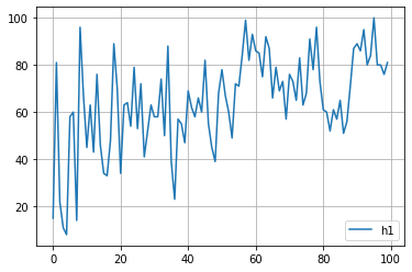
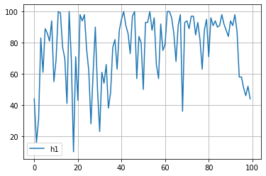
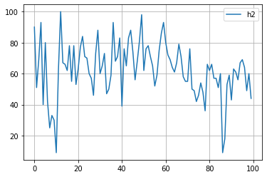
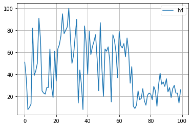
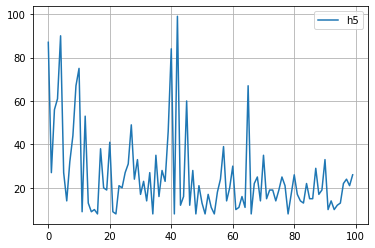
for key in study.trials[0].params.keys():
    plt.plot([trial.params[key] for trial in study.trials], label=key)
    plt.grid()
    plt.legend()
    plt.show()

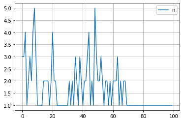
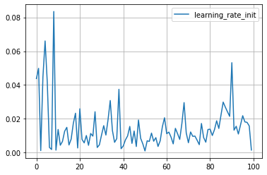
層の深さを固定しない

# 目的関数
def objective(trial):
    h1, = trial.suggest_int('h1', 8, 100),
    h2, = trial.suggest_int('h2', 8, 100),
    h3, = trial.suggest_int('h3', 8, 100),
    h4, = trial.suggest_int('h4', 8, 100),
    h5, = trial.suggest_int('h5', 8, 100),
    hidden_layer_sizes = []
    n = trial.suggest_int('n', 1, 5)
    for h in [h1, h2, h3, h4, h5]:
        hidden_layer_sizes.append(h)
        if len(hidden_layer_sizes) == n:
            break
    learning_rate_init, = trial.suggest_loguniform('learning_rate_init', 0.001, 0.1),
    classifier = MLPClassifier(max_iter=10000, early_stopping=True,
                                    hidden_layer_sizes=hidden_layer_sizes,
                                    learning_rate_init=learning_rate_init, 
                                    solver='adam', activation='relu')
    classifier.fit(X_train, y_train)
    #return classifier.score(X_train, y_train)
    #return classifier.score(X_test, y_test)
    return np.linalg.norm(y_train - classifier.predict_proba(X_train)[:, 1], ord=1)

#study = optuna.create_study(direction='maximize')
study = optuna.create_study(direction='minimize')
study.optimize(objective, n_trials=100)

[32m[I 2019-12-13 00:34:37,028][0m Finished trial#0 resulted in value: 117.6950339936551. Current best value is 117.6950339936551 with parameters: {'h1': 44, 'h2': 90, 'h3': 75, 'h4': 51, 'h5': 87, 'n': 3, 'learning_rate_init': 0.043829528929494495}.[0m
[32m[I 2019-12-13 00:34:37,247][0m Finished trial#1 resulted in value: 107.63845860162616. Current best value is 107.63845860162616 with parameters: {'h1': 16, 'h2': 51, 'h3': 13, 'h4': 36, 'h5': 27, 'n': 3, 'learning_rate_init': 0.04986625228277607}.[0m
[32m[I 2019-12-13 00:34:37,513][0m Finished trial#2 resulted in value: 198.86827020586986. Current best value is 107.63845860162616 with parameters: {'h1': 16, 'h2': 51, 'h3': 13, 'h4': 36, 'h5': 27, 'n': 3, 'learning_rate_init': 0.04986625228277607}.[0m
...（中略）...
[32m[I 2019-12-13 00:35:10,424][0m Finished trial#97 resulted in value: 31.485260318520005. Current best value is 23.024826770529504 with parameters: {'h1': 62, 'h2': 60, 'h3': 58, 'h4': 77, 'h5': 27, 'n': 1, 'learning_rate_init': 0.011342241271350882}.[0m
[32m[I 2019-12-13 00:35:10,801][0m Finished trial#98 resulted in value: 27.752591077771235. Current best value is 23.024826770529504 with parameters: {'h1': 62, 'h2': 60, 'h3': 58, 'h4': 77, 'h5': 27, 'n': 1, 'learning_rate_init': 0.011342241271350882}.[0m
[32m[I 2019-12-13 00:35:11,199][0m Finished trial#99 resulted in value: 81.29419572506973. Current best value is 23.024826770529504 with parameters: {'h1': 62, 'h2': 60, 'h3': 58, 'h4': 77, 'h5': 27, 'n': 1, 'learning_rate_init': 0.011342241271350882}.[0m

study.best_params

{'h1': 62,
 'h2': 60,
 'h3': 58,
 'h4': 77,
 'h5': 27,
 'learning_rate_init': 0.011342241271350882,
 'n': 1}

study.best_value

23.024826770529504

plt.plot([trial.value for trial in study.trials], label='score')
plt.grid()
plt.legend()
plt.show()

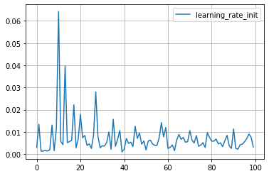
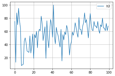
for key in study.trials[0].params.keys():
    plt.plot([trial.params[key] for trial in study.trials], label=key)
    plt.grid()
    plt.legend()
    plt.show()

PyTorch + Optuna

上記と同じように、多層パーセプトロンの最適化を PyTorch + Optuna で試してみました。

import torch
from torch.utils.data import TensorDataset
from torch.utils.data import DataLoader

X_train = torch.from_numpy(X_train).float()
X_test = torch.from_numpy(X_test).float()
y_train = torch.from_numpy(y_train).float()
y_test = torch.from_numpy(y_test).float()

train = TensorDataset(X_train, y_train)

train_loader = DataLoader(train, batch_size=10, shuffle=True)

import torch
class MLPC(torch.nn.Module):
    def __init__(self, n_input, n_hidden1, n_output):
        super(MLPC, self).__init__()
        self.l1 = torch.nn.Linear(n_input, n_hidden1)
        self.l2 = torch.nn.Linear(n_hidden1, n_output)

    def forward(self, x):
        h1 = self.l1(x)
        h2 = torch.sigmoid(h1)
        h3 = self.l2(h2)
        h4 = torch.sigmoid(h3)
        return h4

    def score(self, x, y, threshold=0.5):
        accum = 0
        for y_pred, y1 in zip(self.forward(x), y):
            if y1 == 1:
                if y_pred >= threshold:
                    accum += 1
            else:
                if y_pred < threshold:
                    accum += 1
        return accum / len(y)

# 目的関数
from torch.autograd import Variable
def objective(trial):
    n_h1, = trial.suggest_int('n_hidden1', 1, 100),
    lr, = trial.suggest_loguniform('lr', 0.001, 0.1),
    model = MLPC(len(train[0][0]), n_h1, 1)
    criterion = torch.nn.MSELoss()
    optimizer = torch.optim.SGD(model.parameters(), lr=lr)

    #loss_history = []
    n_epoch = 2000
    for epoch in range(n_epoch):
        total_loss = 0
        for x, y in train_loader:
            x = Variable(x)
            y = Variable(y)
            optimizer.zero_grad()
            y_pred = model(x)
            loss = criterion(y_pred, y)
            loss.backward()
            optimizer.step()
            total_loss += loss.item()
        #loss_history.append(total_loss)
        #if (epoch +1) % (n_epoch / 10) == 0:
        #    print(epoch + 1, total_loss)
    score_train_history.append(model.score(X_train, y_train))
    score_test_history.append(model.score(X_test, y_test))
    return total_loss # model.score(X_test, y_test) にすると学習が進まない？

失敗編

n_trials=100
score_train_history = []
score_test_history = []
study = optuna.create_study(direction='minimize')
study.optimize(objective, n_trials=n_trials)

/usr/local/lib/python3.6/dist-packages/torch/nn/modules/loss.py:431: UserWarning:

Using a target size (torch.Size([10])) that is different to the input size (torch.Size([10, 1])). This will likely lead to incorrect results due to broadcasting. Please ensure they have the same size.

/usr/local/lib/python3.6/dist-packages/torch/nn/modules/loss.py:431: UserWarning:

Using a target size (torch.Size([1])) that is different to the input size (torch.Size([1, 1])). This will likely lead to incorrect results due to broadcasting. Please ensure they have the same size.

[32m[I 2019-12-13 00:36:09,957][0m Finished trial#0 resulted in value: 8.354197099804878. Current best value is 8.354197099804878 with parameters: {'n_hidden1': 50, 'lr': 0.008643921209550006}.[0m
[32m[I 2019-12-13 00:37:02,256][0m Finished trial#1 resulted in value: 8.542565807700157. Current best value is 8.354197099804878 with parameters: {'n_hidden1': 50, 'lr': 0.008643921209550006}.[0m
[32m[I 2019-12-13 00:37:54,087][0m Finished trial#2 resulted in value: 8.721126735210419. Current best value is 8.354197099804878 with parameters: {'n_hidden1': 50, 'lr': 0.008643921209550006}.[0m
...（中略）...
[32m[I 2019-12-13 01:59:43,405][0m Finished trial#97 resulted in value: 8.414046227931976. Current best value is 8.206612035632133 with parameters: {'n_hidden1': 82, 'lr': 0.0010109929013465883}.[0m
[32m[I 2019-12-13 02:00:36,203][0m Finished trial#98 resulted in value: 8.469094559550285. Current best value is 8.206612035632133 with parameters: {'n_hidden1': 82, 'lr': 0.0010109929013465883}.[0m
[32m[I 2019-12-13 02:01:28,698][0m Finished trial#99 resulted in value: 8.296677514910698. Current best value is 8.206612035632133 with parameters: {'n_hidden1': 82, 'lr': 0.0010109929013465883}.[0m

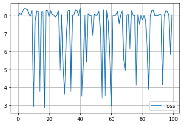
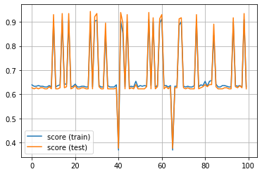
まずは失敗編です。なにか Warning が出ましたね。気にせず続けてみましたが、警告通り、精度は上がりませんでした。

study.best_params

{'lr': 0.0010109929013465883, 'n_hidden1': 82}

study.best_value

8.206612035632133

plt.plot([trial.value for trial in study.trials], label='loss')
plt.grid()
plt.legend()
plt.show()

plt.plot(score_train_history, label='score (train)')
plt.plot(score_test_history, label='score (test)')
plt.grid()
plt.legend()
plt.show()

for key in study.trials[0].params.keys():
    plt.plot([trial.params[key] for trial in study.trials], label=key)
    plt.grid()
    plt.legend()
    plt.show()

成功編

上の「失敗編」は、何がまずかったのでしょうか？ 警告メッセージ

/usr/local/lib/python3.6/dist-packages/torch/nn/modules/loss.py:431: UserWarning:

Using a target size (torch.Size([10])) that is different to the input size (torch.Size([10, 1])). This will likely lead to incorrect results due to broadcasting. Please ensure they have the same size.

/usr/local/lib/python3.6/dist-packages/torch/nn/modules/loss.py:431: UserWarning:

Using a target size (torch.Size([1])) that is different to the input size (torch.Size([1, 1])). This will likely lead to incorrect results due to broadcasting. Please ensure they have the same size.

の意味は、目的変数の行列の形が良くないということです。今回は、

# https://scikit-learn.org/stable/modules/generated/sklearn.datasets.load_breast_cancer.html
from sklearn.datasets import load_breast_cancer
breast_cancer = load_breast_cancer()
X = breast_cancer.data
y = breast_cancer.target

のようにして説明変数と目的変数を作成しましたが、このときの y を reshape する必要があります。

y = y.reshape((len(y), 1))

失敗の原因はこれだけでした。それ以外は、さっきと全く同じコードで精度が上がりました。失敗の時と比べてみましょう。

# 訓練データとテストデータに分割するメソッドのインポート
from sklearn.model_selection import train_test_split 
# 訓練データ・テストデータへ6:4の比でランダムに分割
X_train, X_test, y_train, y_test = train_test_split(X, y, test_size=.4) 

import torch
from torch.utils.data import TensorDataset
from torch.utils.data import DataLoader

X_train = torch.from_numpy(X_train).float()
X_test = torch.from_numpy(X_test).float()
y_train = torch.from_numpy(y_train).float()
y_test = torch.from_numpy(y_test).float()

train = TensorDataset(X_train, y_train)

train_loader = DataLoader(train, batch_size=10, shuffle=True)

import torch
class MLPC(torch.nn.Module):
    def __init__(self, n_input, n_hidden1, n_output):
        super(MLPC, self).__init__()
        self.l1 = torch.nn.Linear(n_input, n_hidden1)
        self.l2 = torch.nn.Linear(n_hidden1, n_output)

    def forward(self, x):
        h1 = self.l1(x)
        h2 = torch.sigmoid(h1)
        h3 = self.l2(h2)
        h4 = torch.sigmoid(h3)
        return h4

    def score(self, x, y, threshold=0.5):
        accum = 0
        for y_pred, y1 in zip(self.forward(x), y):
            if y1 == 1:
                if y_pred >= threshold:
                    accum += 1
            else:
                if y_pred < threshold:
                    accum += 1
        return accum / len(y)

# 目的関数
from torch.autograd import Variable
def objective(trial):
    n_h1, = trial.suggest_int('n_hidden1', 1, 100),
    lr, = trial.suggest_loguniform('lr', 0.001, 0.1),
    model = MLPC(len(train[0][0]), n_h1, 1)
    criterion = torch.nn.MSELoss()
    optimizer = torch.optim.SGD(model.parameters(), lr=lr)

    #loss_history = []
    n_epoch = 2000
    for epoch in range(n_epoch):
        total_loss = 0
        for x, y in train_loader:
            #if x.shape[0] == 1:
            #    continue
            #print(x.shape, y.shape)
            x = Variable(x)
            y = Variable(y)
            optimizer.zero_grad()
            y_pred = model(x)
            loss = criterion(y_pred, y)
            loss.backward()
            optimizer.step()
            total_loss += loss.item()
        #loss_history.append(total_loss)
        #if (epoch +1) % (n_epoch / 10) == 0:
        #    print(epoch + 1, total_loss)
    score_train_history.append(model.score(X_train, y_train))
    score_test_history.append(model.score(X_test, y_test))
    return total_loss # model.score(X_test, y_test) にすると学習が進まない?

n_trials=100
score_train_history = []
score_test_history = []
study = optuna.create_study(direction='minimize')
study.optimize(objective, n_trials=n_trials)

[32m[I 2019-12-13 07:58:42,273][0m Finished trial#0 resulted in value: 7.991558387875557. Current best value is 7.991558387875557 with parameters: {'n_hidden1': 100, 'lr': 0.001719688534454947}.[0m
[32m[I 2019-12-13 07:59:29,221][0m Finished trial#1 resulted in value: 8.133784644305706. Current best value is 7.991558387875557 with parameters: {'n_hidden1': 100, 'lr': 0.001719688534454947}.[0m
[32m[I 2019-12-13 08:00:16,849][0m Finished trial#2 resulted in value: 8.075047567486763. Current best value is 7.991558387875557 with parameters: {'n_hidden1': 100, 'lr': 0.001719688534454947}.[0m
...（中略）...
[32m[I 2019-12-13 09:14:47,236][0m Finished trial#97 resulted in value: 8.02999284863472. Current best value is 2.8610200360417366 with parameters: {'n_hidden1': 38, 'lr': 0.0010151912634053866}.[0m
[32m[I 2019-12-13 09:15:34,106][0m Finished trial#98 resulted in value: 5.849344417452812. Current best value is 2.8610200360417366 with parameters: {'n_hidden1': 38, 'lr': 0.0010151912634053866}.[0m
[32m[I 2019-12-13 09:16:20,332][0m Finished trial#99 resulted in value: 8.052950218319893. Current best value is 2.8610200360417366 with parameters: {'n_hidden1': 38, 'lr': 0.0010151912634053866}.[0m

study.best_params

{'lr': 0.0010151912634053866, 'n_hidden1': 38}

study.best_value

2.8610200360417366

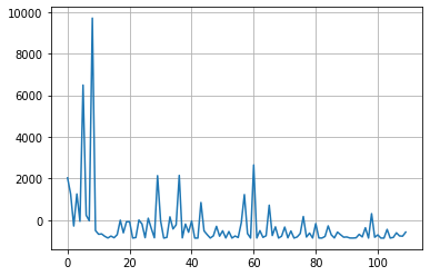
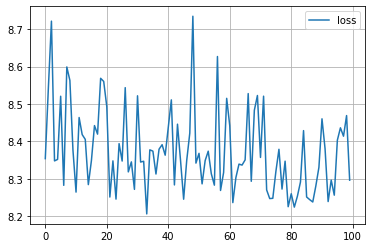
%matplotlib inline
import matplotlib.pyplot as plt
plt.plot([trial.value for trial in study.trials], label='loss')
plt.grid()
plt.legend()
plt.show()

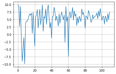
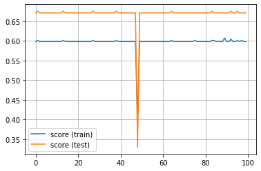
plt.plot(score_train_history, label='score (train)')
plt.plot(score_test_history, label='score (test)')
plt.grid()
plt.legend()
plt.show()

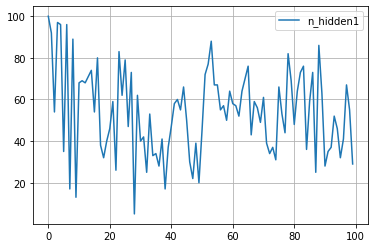
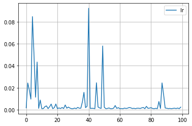
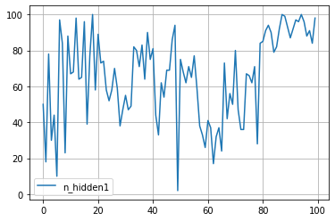
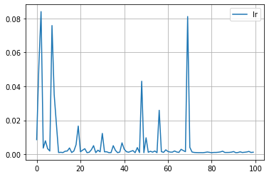
for key in study.trials[0].params.keys():
    plt.plot([trial.params[key] for trial in study.trials], label=key)
    plt.grid()
    plt.legend()
    plt.show()