機械学習でギターアンプをモデリングするを参考にしながら,nnablaでの学習モデルを作成していきたい。
モデル検討
前回構築した環境でまずnnablaでLSTMの実装を確認してみる。
使うかどうかわからないが、nnabla-c-runtimeではLSTMレイヤーのサポートはされていないようだ。
※最新の1.6ではPython上でのLSTMレイヤーのCPU演算に対応したようだ。もともとGPUのみの対応だったとのこと
既存のLSTMレイヤーはそのまま使うと制約がいくつかあるようだ。
いろいろ調べていると、LSTMレイヤーをベーシックな関数で構築すれば制約の問題はクリアできそう。
nnablaでLSTMモデルを作成する際、Neural Network ConsoleというWindowsGUIで、LSTMの実装例があるので確認してみる。

上記からpythonのコードにエクスポートすることもできる。
今更聞けないLSTMの基本にあるLSTMの基本構造をそのまま表現している。
上記は、Neural Network Console内のlong_short_term_memory(LSTM)というチュートリアルで、
MNISTデータセットの“4”と“9”の28x28ピクセルデータを長さ28、バッチサイズ28にばらしてrecurrentinput~recurrentoutputを28回回した結果を活性化関数を通して4だったら0,
9だったら1という風に判定するサンプルである。
今回のLSTM計算は、上記や、過去の株価から未来時間x点の株価予測、サイン波の入力から未来時間x点の値のような問題ではなく、入力の長さに対して出力の長さが同じ音声データで、その2つの平均二乗誤差(MSE)を評価する計算となるので、Keras LSTMでいうところのreturn_sequences=Trueの実装が重要となる。
nnablaでその点を意識したサンプルがNNablaでLSTMの実装としてあるので、参考、引用させてもらいながらいろいろ検討して下記のようにモデルを作った。
def LSTMCell(x , h2, h1):

    units = h1.shape[1]

    # h2=hidden, h1= cell
    h2 = F.concatenate(h2, x, axis=1)

    h3 = PF.affine(h2, ( units), name='Affine')

    h4 = PF.affine(h2, ( units), name='InputGate')

    h5 = PF.affine(h2, ( units), name='ForgetGate')

    h6 = PF.affine(h2, ( units), name='OutputGate')

    h3 = F.tanh(h3)

    h4 = F.sigmoid(h4)

    h5 = F.sigmoid(h5)

    h6 = F.sigmoid(h6)

    h4 = F.mul2(h4, h3)

    h5 = F.mul2(h5, h1)

    h4 = F.add2(h4, h5, True)

    h7 = F.tanh(h4)

    h6 = F.mul2(h6, h7)

    return h6 , h4 # hidden, cell


def LSTM(inputs, units, initial_state=None, return_sequences=False, return_state=False, name='lstm'):

    batch_size = inputs.shape[0]

    if initial_state is None:

        c0 = nn.Variable.from_numpy_array(np.zeros((batch_size, units)), need_grad=True)
        h0 = nn.Variable.from_numpy_array(np.zeros((batch_size, units)), need_grad=True)
    else:
        assert type(initial_state) is tuple or type(initial_state) is list, \
               'initial_state must be a typle or a list.'
        assert len(initial_state) == 2, \
               'initial_state must have only two states.'

        c0, h0 = initial_state

        assert c0.shape == h0.shape, 'shapes of initial_state must be same.'
        assert c0.shape[0] == batch_size, \
               'batch size of initial_state ({0}) is different from that of inputs ({1}).'.format(c0.shape[0], batch_size)
        assert c0.shape[1] == units, \
               'units size of initial_state ({0}) is different from that of units of args ({1}).'.format(c0.shape[1], units)

    cell = c0
    hidden = h0

    hs = []

    for x in F.split(inputs, axis=1):
        with nn.parameter_scope(name):
            cell, hidden = LSTMCell(x, cell, hidden)
        hs.append(hidden)

    if return_sequences:
        ret = F.stack(*hs, axis=1)
    else:
        ret = hs[-1]

    if return_state:
        return ret, cell, hidden
    else:
        return ret


def build_model(x):
    t = LSTM(x, 16,  return_sequences=True, name='LSTM1')
    t2 = LSTM(t, 1,  return_sequences=True, name='LSTM_OUT')
    return t2
これで学習モデルが完成した。
NNablaへの実装
学習ファイルのイテレーターの作成
機械学習でギターアンプをモデリングするから引用させていただいた。
バッチの作成
config.ymlは下記の設定とした。
input_timesteps: 960
output_timesteps: 480
batch_size: 64

これにより、学習時は、イテレーターから960サンプル×64=61,440サンプルのドライ音、ウェット音を取り出し、おしりの480×64=30,720サンプルでロス関数作成を行う。
イテレーターは、
    train_dataset = [
        (load_wave(_[0]).reshape(-1, 1), load_wave(_[1]).reshape(-1, 1))
        for _ in config["train_data"]]
    train_dataflow = flow(train_dataset, input_timesteps, batch_size)
とし、NNablaの専用変数nn.valiableを作成しモデルに代入、
x = nn.Variable((batch_size, input_timesteps, 1), need_grad=True)
y = nn.Variable((batch_size, input_timesteps, 1), need_grad=True)
中間層セル数は、上記の学習モデル内に設定した通り、いったん1段目は16セル、2段目は1セルで出力とし、上記をバッチサイズ、シーケンス長、次元の順番にアレイにして、説明変数とする。
    t = build_model(x)

    ロス関数作成
    loss = F.mean(F.squared_error(t[:, -output_timesteps:, :], y[:, -output_timesteps:, :]))
これを追い込むソルバーはadaboundを使用。
    solver = S.AdaBound()
        solver.set_parameters(nn.get_parameters(grad_only=False))
とする。
NNabla学習ルーチン
学習ルーチンはエポック全体を回すが、1エポックごとにh5ファイルへ学習データを吐き出す設定。
1エポック当たり100ステップ、10回の検証を行う設定。
ベストなロス関数結果が出なくなったら自動で止まるアーリーストッピング、進捗を見るtqdm、学習の進行具合を見るtensorboardを組み込んだ。
    es = EarlyStopping(patience=patience)

    steps = 100
    validation_time = 10


    cp_dir = "checkpoint/{:%Y%m%d_%H%M%S}".format(timestamp)
    if not os.path.exists(cp_dir):
        os.makedirs(cp_dir)

    idx = 0

    for i in tloop:

        # TRAINING

        tloop.set_description("Training Epoch")
        st = tqdm.trange( 0, steps )
        losses = AverageMeter()
        for j in st:

            x.d ,y.d  = train_dataflow.__next__()
            st.set_description("Training Steps")
            loss.forward()
            solver.zero_grad()
            loss.backward()
            solver.update()
            losses.update(loss.d.copy().mean())
            st.set_postfix(
                train_loss=losses.avg
            )

            # write train graph
            tb_writer.add_scalar('train/loss', losses.avg, global_step=idx)
            idx += 1
学習動作中に、別コンソールで、
tensorboard --logdir=tensorboard/YYYYMMDD_HHMMSS(年月日、時間でフォルダができる)
とやると学習進捗が確認できる。
最終的に学習が終了したグラフが下記。GPUよりCPU演算のほうが倍近く早く終了したため、CPU演算としている。
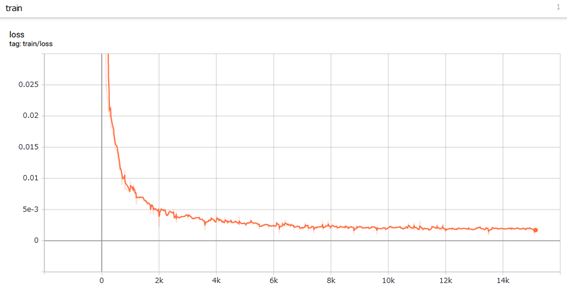
学習は0.0019くらいで収束した模様。
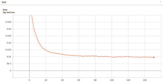
アーリーストッピングが50回設定で0.0091くらいが最小誤差になったようだ。
これでベストな結果が、checkpoint/YYYYMMDD_HHMMSS(年月日、時間でフォルダができる)/best_result.h5として保存される。
この中身をHDFviewで見てみる。

1段目のLSTM、2段目のLSTMが保存されており、中間層セル数の16が反映されているようだ。
このファイルのサイズは32.5kバイトで非常に小さい。
全体のソースコードはGithubにて公開中。