モチベーション
※本記事は以前の記事の誤りを再度訂正するものである。あの記事は問題と誤解がある。
データ分析で分布を調べることは基礎的な手順のひとつであるが、1次データが常に手に入るとは限らない。特に調査会社のレポートはRAWデータなしの分位数データしか手に入らないことも多いはず。分位数のデータから分布を予測する方法をメモ代わりに記しておきたい。さらにはデータ測定には打ち切りがありことや、確率分布が出現する値(台)についても注意を払うべきであろう。
パッケージインストールとデータ読み込み
using Distributions,StatsPlots,Statistics,DataFrames,CSV
using Turing,LinearAlgebra
北海道マラソン2024 完走タイム別人数分布表
今年も北海道マラソンが開催されるので、ひきつづきこれを事例にしてみる。北海道マラソン運営はスタートから10分刻みの完走タイム別人数分布表を公開している。発表データを以下に転記する。報道によると参加者は1万7705人だったので、2562名は完走できなかったようだ。
| タイム範囲 | 男子 | 女子 | オープン | 合計 |
|---|---|---|---|---|
| 2:10:01~2:20:00 | 10 | 0 | 0 | 10 |
| 2:20:01~2:30:00 | 19 | 0 | 0 | 19 |
| 2:30:01~2:40:00 | 34 | 6 | 0 | 40 |
| 2:40:01~2:50:00 | 92 | 4 | 0 | 96 |
| 2:50:01~3:00:00 | 152 | 12 | 0 | 164 |
| 3:00:01~3:10:00 | 174 | 14 | 1 | 189 |
| 3:10:01~3:20:00 | 326 | 19 | 2 | 347 |
| 3:20:01~3:30:00 | 446 | 43 | 1 | 490 |
| 3:30:01~3:40:00 | 416 | 52 | 2 | 470 |
| 3:40:01~3:50:00 | 506 | 77 | 4 | 587 |
| 3:50:01~4:00:00 | 731 | 102 | 5 | 838 |
| 4:00:01~4:10:00 | 612 | 103 | 5 | 720 |
| 4:10:01~4:20:00 | 694 | 111 | 11 | 816 |
| 4:20:01~4:30:00 | 816 | 142 | 9 | 967 |
| 4:30:01~4:40:00 | 796 | 154 | 14 | 964 |
| 4:40:01~4:50:00 | 799 | 168 | 24 | 991 |
| 4:50:01~5:00:00 | 920 | 248 | 31 | 1,199 |
| 5:00:01~5:10:00 | 658 | 189 | 18 | 865 |
| 5:10:01~5:20:00 | 791 | 229 | 24 | 1,044 |
| 5:20:01~5:30:00 | 832 | 197 | 30 | 1,059 |
| 5:30:01~5:40:00 | 821 | 224 | 49 | 1,094 |
| 5:40:01~5:50:00 | 863 | 253 | 59 | 1,175 |
| 5:50:01~ | 780 | 179 | 40 | 999 |
| 男子 | 女子 | オープン | 完走者合計 | 未完走者 | 出走者 |
|---|---|---|---|---|---|
| 12,288 | 2,526 | 329 | 15,143 | 2,562 | 17,705 |
完走者の度数表を作成する
df = CSV.read("hokkaido-marason_2024.csv",DataFrame)
df.ac_male = accumulate(+, df[:,:male])
df.ac_female = accumulate(+, df[:,:female])
runner = df[:,:male] .+ df[:,:female] .+ df[:, :open]
df.ac_runner = accumulate(+, runner)
df.percentile_runner = df.ac_runner ./ 17705 #出走者全員
グラフからWeibull分布を仮定する
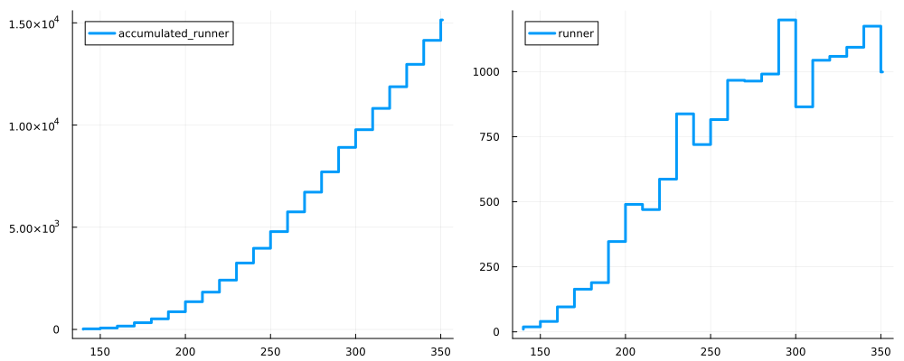
マラソン記録は低いタイムが多く存在し、高い記録が少ない。そのため分布は左右対称ではない。ここではWeibull分布を想定してみたい。Weibull分布は故障率で使われることが多いが、本質的にはある出来ことが成就(完成だったり故障だったり)するまでの時間分布と考えることができる。また記録は6時間(360分)で打ち切りが設定されていることも注意しなければならない。
p1 = @df df plot(st=:steppre,:goal_time,[:ac_male,:ac_female], label=["ac_male" "ac_female"], lw=3)
p2 = @df df plot(st=:steppre,:goal_time,[:male,:female], label=["male" "female"], lw=3)
plot(p1,p2, size=(1000,400))
モデルの作成
モデルに渡すデータは時間区分と度数分布のVectorデータである。Weibull分布の台は0~有限時間であることに対して、マラソンの記録は何らかの物理的な制約がある。世界記録でも2時間を切るのはしばらく先になりそうだし。したがってモデルには物理的な障壁(lm)も推定させる必要がありそうだ。もしくは測定の下限である170分を引いたデータを渡すこともありだろう。また測定打ち切り(u_limit)が6時間(360分)に設定されていることも反映している。
@model function fqweibull(tim, acc ; u_limt=360, n=length(tim), )
    lm ~ truncated(TDist(3), 60, 230)
    a ~ truncated(TDist(2), 1e-3, Inf)
    θ ~ InverseGamma(2,3)
    s ~ Exponential(1)
    dist = truncated(Weibull(a, θ) ; upper = u_limt)
    tim ~ arraydist([Normal(quantile(dist, q) + lm, s ) for q in acc])
end
Turingでパラメータを探す
モデルが作成されたらNUTS()でサンプリングを行う。
times =df[1:(end-1),:goal_time]
quant =df[1:(end-1),:percentile_runner]
c_quantile = sample(fqweibull(times,quant),NUTS(),3000)
Chains MCMC chain (3000×4×1 Array{Float64, 3}):
Iterations        = 1001:1:4000
Number of chains  = 1
Samples per chain = 3000
Wall duration     = 3.03 seconds
Compute duration  = 3.03 seconds
parameters        = lm, a, θ, s
internals         =

Summary Statistics
  parameters       mean       std      mcse   ess_bulk    ess_tail      rhat   ess_per_sec
      Symbol    Float64   Float64   Float64    Float64     Float64   Float64       Float64

          lm   124.9373    2.0190    0.0683   874.4969   1292.3242    0.9997      288.7081
           a     3.1006    0.0649    0.0021   949.3115   1440.3143    0.9998      313.4076
           θ   196.6165    2.0047    0.0651   944.0560   1122.7947    0.9997      311.6725
           s     1.7503    0.2972    0.0091   996.7565    666.3171    1.0002      329.0711

Quantiles
  parameters       2.5%      25.0%      50.0%      75.0%      97.5%
      Symbol    Float64    Float64    Float64    Float64    Float64

          lm   120.9525   123.5922   124.9787   126.2671   128.7652
           a     2.9765     3.0568     3.1000     3.1432     3.2299
           θ   192.7589   195.2666   196.5504   197.9681   200.5981
           s     1.2656     1.5438     1.7121     1.9214     2.4396
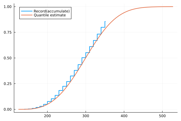
推定結果をグラフ化して比較してみる
わりとうまくフィットした感じがする。
runner_param = get(c_quantile,[:a, :θ]) |> t-> (mean(t.a), mean(t.θ))
runner_lm = get(c_quantile,[:lm]) |> t-> mean(t.lm)
@df df plot(:goal_time , :percentile_runner, st=:steppre, label="Record(accumulate)",lw=2,legend=:topleft)
plot!(Weibull(runner_param...) .+ runner_lm ,func=cdf,lw=2,label="Quantile estimate")
ランナーの性別記録は正確な度数がわからない
性別データも同じくできればいいが、実際は未完走者が2,562名(約15%)おり、その一部が男性であろうという情報だけなので、男性の出走者数(完走者じゃないよ)がわからないのである。未完走者は何かしらの事情で非常に長い時間がかかってしまった人とみなすなら、この情報をモデルに組み込むことができる。
【変更点】
・おおよそ未完走者の割合は15%程度
・入力データとして累積時間別の人数を渡し、モデル内で計算
・Weibullの切り捨て(Truncated)をやめて、未完走者は測定時間幅の右側外と考える
・完走者合計(goal_sum)を因数として渡す
@model function fqweibull(tim, acx , goal_sum ; u_limt=360, n=length(tim))
    #未完走者推定
    retire ~ truncated( Normal( 0.15 *  (12288/(1 - 0.15)), 1000) , 0, 2562)
    ac_quant = [ ac / (retire + goal_sum) for ac in acx]
    lm ~ truncated(TDist(3), 60, 160)
    a ~ truncated(TDist(2), 1e-3, Inf)
    θ ~ InverseGamma(2,3)
    s ~ Exponential(1)
#    dist = truncated(Weibull(a, θ) ; upper = u_limt)
    dist = Weibull(a, θ)
    tim ~ arraydist([Normal(quantile(dist, q) + lm, s ) for q in ac_quant])
    return ac_quant
end

times =df[1:(end-1),:goal_time]
ac_xs =df[1:(end-1),:ac_male]
m_chain = sample(fqweibull(times,ac_xs, df.ac_male[end]),NUTS(),3000)
Chains MCMC chain (3000×17×1 Array{Float64, 3}):

Iterations        = 1001:1:4000
Number of chains  = 1
Samples per chain = 3000
Wall duration     = 3.72 seconds
Compute duration  = 3.72 seconds
parameters        = retire, lm, a, θ, s
internals         = lp, n_steps, is_accept, acceptance_rate, log_density, hamiltonian_energy, hamiltonian_energy_error, max_hamiltonian_energy_error, tree_depth, numerical_error, step_size, nom_step_size

Summary Statistics
  parameters        mean        std      mcse    ess_bulk    ess_tail      rhat   ess_per_sec
      Symbol     Float64    Float64   Float64     Float64     Float64   Float64       Float64

      retire   2336.7841   199.2009    4.9968   1272.4537    934.2466    1.0010      342.0574
          lm    123.8325     3.9260    0.1195   1112.8539   1161.1553    1.0010      299.1543
           a      3.0735     0.1262    0.0038   1149.4288   1156.5061    1.0013      308.9862
           θ    194.8638     4.0151    0.1167   1183.7661   1216.4229    1.0010      318.2167
           s      3.2534     0.4987    0.0118   1833.2027   1666.6718    0.9997      492.7964

Quantiles
  parameters        2.5%       25.0%       50.0%       75.0%       97.5%
      Symbol     Float64     Float64     Float64     Float64     Float64

      retire   1839.9728   2232.9428   2392.9250   2491.6245   2556.6401
          lm    115.4712    121.3094    124.0152    126.5734    130.8725
           a      2.8568      2.9851      3.0627      3.1498      3.3475
           θ    187.1262    192.2186    194.8715    197.4774    202.8322
           s      2.4203      2.9071      3.2009      3.5524      4.3799
グラフ化して予測値と実測を比べる
male_param = get(m_chain, [:a, :θ]) |> t-> (mean(t.a), mean(t.θ))
male_lm = get(m_chain,[:lm]) |> t-> mean(t.lm)
male_retire = get(m_chain,[:retire]) |> t-> mean(t.retire)
@df df plot(Weibull(male_param...) .+ male_lm, func=cdf, label="estimate_male", lw=2)
@df df plot!(:goal_time, :ac_male ./ ( :ac_male[end] + male_retire) , st=:steppre, label="ac_male", lw=2)
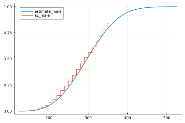
うまく推定できたようだがどうだろう。推定したWeibull分布をつかって95%域を推定することができる。約400分(6時間40分)まで走れるようにすれば、男性出走者の約95%が完走できるようになるかもしれない。
quantile(truncated(Weibull(male_param...), 0, 360), [0.95])[1] + male_lm