はじめに
前回の続きです.実装したコードはここ(https://github.com/jjjkkkjjj/pytorch_SSD)にあります.
モデル
SSD300(
  (codec): Codec(
    (encoder): Encoder()
    (decoder): Decoder()
  )
  (defaultBox): DBoxSSD300Original()
  (predictor): Predictor()
  (inferenceBox): InferenceBox()
  (feature_layers): ModuleDict(
    (convRL1_1): ConvRelu(
      (conv): Conv2d(3, 64, kernel_size=(3, 3), stride=(1, 1), padding=(1, 1))
      (relu): ReLU(inplace=True)
    )
    (convRL1_2): ConvRelu(
      (conv): Conv2d(64, 64, kernel_size=(3, 3), stride=(1, 1), padding=(1, 1))
      (relu): ReLU(inplace=True)
    )
    (pool1): MaxPool2d(kernel_size=(2, 2), stride=(2, 2), padding=0, dilation=1, ceil_mode=False)
    (convRL2_1): ConvRelu(
      (conv): Conv2d(64, 128, kernel_size=(3, 3), stride=(1, 1), padding=(1, 1))
      (relu): ReLU(inplace=True)
    )
    (convRL2_2): ConvRelu(
      (conv): Conv2d(128, 128, kernel_size=(3, 3), stride=(1, 1), padding=(1, 1))
      (relu): ReLU(inplace=True)
    )
    (pool2): MaxPool2d(kernel_size=(2, 2), stride=(2, 2), padding=0, dilation=1, ceil_mode=False)
    (convRL3_1): ConvRelu(
      (conv): Conv2d(128, 256, kernel_size=(3, 3), stride=(1, 1), padding=(1, 1))
      (relu): ReLU(inplace=True)
    )
    (convRL3_2): ConvRelu(
      (conv): Conv2d(256, 256, kernel_size=(3, 3), stride=(1, 1), padding=(1, 1))
      (relu): ReLU(inplace=True)
    )
    (convRL3_3): ConvRelu(
      (conv): Conv2d(256, 256, kernel_size=(3, 3), stride=(1, 1), padding=(1, 1))
      (relu): ReLU(inplace=True)
    )
    (pool3): MaxPool2d(kernel_size=(2, 2), stride=(2, 2), padding=0, dilation=1, ceil_mode=True)
    (convRL4_1): ConvRelu(
      (conv): Conv2d(256, 512, kernel_size=(3, 3), stride=(1, 1), padding=(1, 1))
      (relu): ReLU(inplace=True)
    )
    (convRL4_2): ConvRelu(
      (conv): Conv2d(512, 512, kernel_size=(3, 3), stride=(1, 1), padding=(1, 1))
      (relu): ReLU(inplace=True)
    )
    (convRL4_3): ConvRelu(
      (conv): Conv2d(512, 512, kernel_size=(3, 3), stride=(1, 1), padding=(1, 1))
      (relu): ReLU(inplace=True)
    )
    (pool4): MaxPool2d(kernel_size=(2, 2), stride=(2, 2), padding=0, dilation=1, ceil_mode=False)
    (convRL5_1): ConvRelu(
      (conv): Conv2d(512, 512, kernel_size=(3, 3), stride=(1, 1), padding=(1, 1))
      (relu): ReLU(inplace=True)
    )
    (convRL5_2): ConvRelu(
      (conv): Conv2d(512, 512, kernel_size=(3, 3), stride=(1, 1), padding=(1, 1))
      (relu): ReLU(inplace=True)
    )
    (convRL5_3): ConvRelu(
      (conv): Conv2d(512, 512, kernel_size=(3, 3), stride=(1, 1), padding=(1, 1))
      (relu): ReLU(inplace=True)
    )
    (pool5): MaxPool2d(kernel_size=(3, 3), stride=(1, 1), padding=1, dilation=1, ceil_mode=False)
    (convRL6): ConvRelu(
      (conv): Conv2d(512, 1024, kernel_size=(3, 3), stride=(1, 1), padding=(6, 6), dilation=(6, 6))
      (relu): ReLU(inplace=True)
    )
    (convRL7): ConvRelu(
      (conv): Conv2d(1024, 1024, kernel_size=(1, 1), stride=(1, 1))
      (relu): ReLU(inplace=True)
    )
    (convRL8_1): ConvRelu(
      (conv): Conv2d(1024, 256, kernel_size=(1, 1), stride=(1, 1))
      (relu): ReLU(inplace=True)
    )
    (convRL8_2): ConvRelu(
      (conv): Conv2d(256, 512, kernel_size=(3, 3), stride=(2, 2), padding=(1, 1))
      (relu): ReLU(inplace=True)
    )
    (convRL9_1): ConvRelu(
      (conv): Conv2d(512, 128, kernel_size=(1, 1), stride=(1, 1))
      (relu): ReLU(inplace=True)
    )
    (convRL9_2): ConvRelu(
      (conv): Conv2d(128, 256, kernel_size=(3, 3), stride=(2, 2), padding=(1, 1))
      (relu): ReLU(inplace=True)
    )
    (convRL10_1): ConvRelu(
      (conv): Conv2d(256, 128, kernel_size=(1, 1), stride=(1, 1))
      (relu): ReLU(inplace=True)
    )
    (convRL10_2): ConvRelu(
      (conv): Conv2d(128, 256, kernel_size=(3, 3), stride=(1, 1))
      (relu): ReLU(inplace=True)
    )
    (convRL11_1): ConvRelu(
      (conv): Conv2d(256, 128, kernel_size=(1, 1), stride=(1, 1))
      (relu): ReLU(inplace=True)
    )
    (convRL11_2): ConvRelu(
      (conv): Conv2d(128, 256, kernel_size=(3, 3), stride=(1, 1))
      (relu): ReLU(inplace=True)
    )
  )
  (addon_layers): ModuleDict(
    (addon_1): L2Normalization()
  )
  (localization_layers): ModuleDict(
    (conv_loc_1): Conv2d(512, 16, kernel_size=(3, 3), stride=(1, 1), padding=(1, 1))
    (conv_loc_2): Conv2d(1024, 24, kernel_size=(3, 3), stride=(1, 1), padding=(1, 1))
    (conv_loc_3): Conv2d(512, 24, kernel_size=(3, 3), stride=(1, 1), padding=(1, 1))
    (conv_loc_4): Conv2d(256, 24, kernel_size=(3, 3), stride=(1, 1), padding=(1, 1))
    (conv_loc_5): Conv2d(256, 16, kernel_size=(3, 3), stride=(1, 1), padding=(1, 1))
    (conv_loc_6): Conv2d(256, 16, kernel_size=(3, 3), stride=(1, 1), padding=(1, 1))
  )
  (confidence_layers): ModuleDict(
    (conv_conf_1): Conv2d(512, 84, kernel_size=(3, 3), stride=(1, 1), padding=(1, 1))
    (conv_conf_2): Conv2d(1024, 126, kernel_size=(3, 3), stride=(1, 1), padding=(1, 1))
    (conv_conf_3): Conv2d(512, 126, kernel_size=(3, 3), stride=(1, 1), padding=(1, 1))
    (conv_conf_4): Conv2d(256, 126, kernel_size=(3, 3), stride=(1, 1), padding=(1, 1))
    (conv_conf_5): Conv2d(256, 84, kernel_size=(3, 3), stride=(1, 1), padding=(1, 1))
    (conv_conf_6): Conv2d(256, 84, kernel_size=(3, 3), stride=(1, 1), padding=(1, 1))
  )
)
このモデルがすること・なすことは以下のようになります.順を追って説明します.
- データセット
- データセットの読み込み
- Augmentation
- Transform(入力画像の前処理)
- Target_transform(正解ラベルの前処理)
- 入力データ
- 正規化済みの$[0,1]$のRGB画像(ここまで前回で説明済み)
- Default Box
-
予測するもの
- Default Boxとのオフセット値→バウンディングボックスの位置
- ラベル
-
学習の流れ
- Default Boxの作成
- 正解ラベルのバウンディングボックスをDefault Boxに割り当て(matching strategy)
- 正解ラベルの正規化!!
- 画像,正解ラベルを入力
- localization lossとconfidence loss(hard negative mining)の計算
テストの流れ- Default Boxの作成
- 画像を入力
- Default Boxとのオフセット値とラベルを予測
- 余分なBoxを除去(Non maximum suppression)
Default Box
物体のバウンディングボックスを予測するためにDefault Box(他にもPrior Box, Anchor Boxとも呼ばれる)なるものを用意します.Default Boxとは,その名の通り事前にデフォルトで存在するBoxのことです.物体検出においてバウンディングボックスの形は無数に候補があって,それを予測するのは骨が折れます.それなら,事前にある程度のDefault Boxを用意して,そのDefault Boxとのオフセット値を回帰する問題にしようとしたわけです.
ここらへんの話は「物体検出についての歴史まとめ」で詳細にまとめられています.
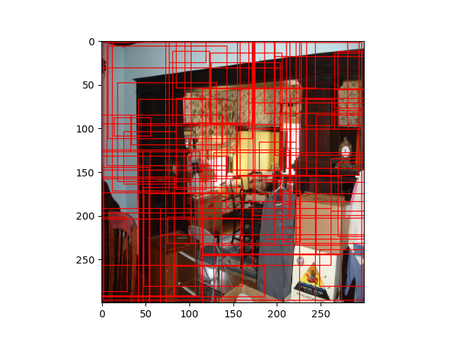
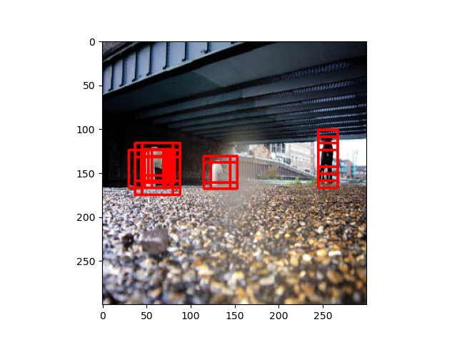
後述ですが,SSD300の場合,Default Boxの数は8732個です(下図はランダムに70個表示したもの,その他はこっち).
予測するもの
- Default Boxとのオフセット値→バウンディングボックスの位置
上述の8732個の$i$番目のDefault Boxに対するオフセット値
(\hat{g}_i^{c_x},\hat{g}_i^{c_y},\hat{g}_i^{w},\hat{g}_i^{h})
を予測します.
- クラスラベル
上述の8732個の$i$番目のDefault Boxに対するクラスラベルの信頼度
\hat{c}_i^{p}
を予測します.ただし,$p$は背景を含めたclass_nums+1個の予測になります.
つまり,1個のDefault Boxに対して,4+class_nums+1個の値を予測することになります.
学習の流れ
Default Boxの作成
作成の流れ
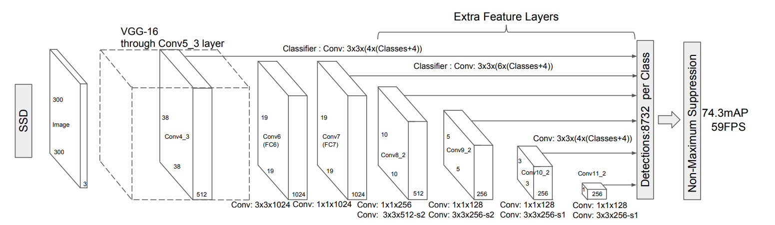
以上を踏まえて,じゃあどうやってDefault Boxを作成するかを説明します.再掲ですが,SSD300のモデルは以下です.
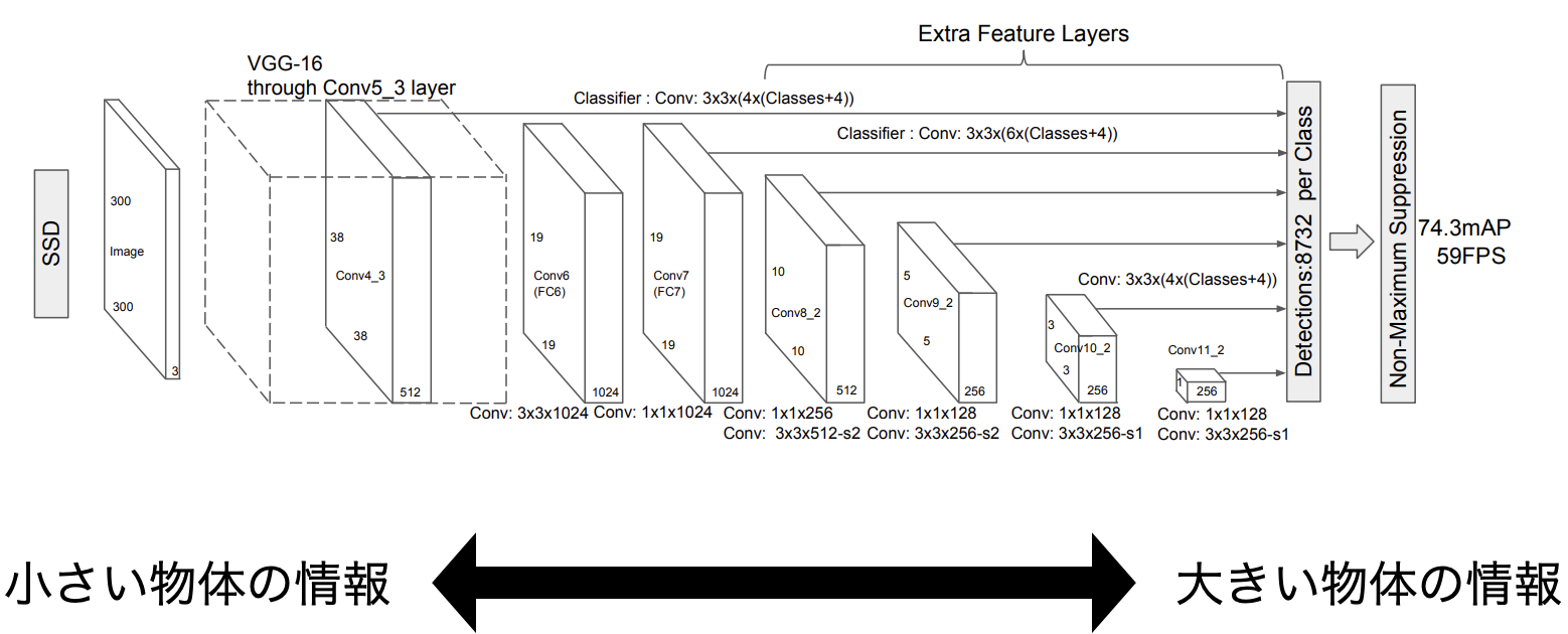
ご覧の通り,入力画像がどんどん圧縮されて最終的には1x1のサイズまで圧縮されていることがわかります.ここで重要なのは,序盤の層は近傍の画素を圧縮しているので,小さい物体の情報を,終盤の層はいろいろな画素を圧縮しているので,大きな物体の情報を持っていると考えることができるということです.
SSD300では,入力から近い順にConv4_3,Conv7,Conv8_2,Conv9_2,Conv10_2,Conv11_2を「予測するDefault Boxのオフセット値」の大元となる特徴マップとします.したがって,これらの特徴マップと対応するDefault Boxを作ることにすれば,Conv4_3[^1]は小さい物体,順に辿って最終的にConv11_2が大きい物体を表していると考えられるので,対応するDefault Boxの大きさもConv4_3から順に大きくなれば良いわけです.したがって,スケール(入力画像に対するDefault Boxの大きさのスケール)を求める式を以下のようにすると,対応するDefault Boxの大きさが順に大きくなります.具体的な数値は順伝搬(L2Normalization)を参照.
$$s_k=s_{min}+\frac{s_{max}-s_{min}}{m-1}(k-1) \tag{1}$$
また,すべての物体が1:1の正方形ではないので,アスペクト比$a$をいくつか用意します.原論文では,アスペクト比$a$は$a_r$とその逆数$a'_r$のどれかとし,
$$a_r \in \{1,2,3\}, a'_r \in \{\frac{1}{1},\frac{1}{2},\frac{1}{3}\}$$
これらを用いて,Default Boxの幅$w_k^a$・高さ$h_k^a$を
$$w_k^a=s_k\sqrt{a},h_k^a=\frac{s_k}{\sqrt{a}}$$
求めています.このとき,$a=\frac{1}{1}$のときは,
s'_k=\sqrt{s_{k}s_{k+1}}
として,ダブリを防ぎます.
※$a$の数が特徴マップの1pixelあたりのDefault Boxの数になります.$a \in \{1,2,\frac{1}{1},\frac{1}{2}\}=\mathbb{A}$のとき,4個となります.
SSD300では,特徴マップのサイズは入力画像が300x300のとき,順に38x38(Conv4_3),19x19(Conv7),10x10(Conv8_2),5x5(Conv9_2),3x3(Conv10_2),1x1(Conv11_2)で,それらに対応するDefault Boxの数は$4=|\mathbb{A} = \{1,2,\frac{1}{1},\frac{1}{2}\}|$,$6=|\mathbb{A} = \{1,2,3,\frac{1}{1},\frac{1}{2},\frac{1}{3}\}|$,$6=|\mathbb{A} = \{1,2,3,\frac{1}{1},\frac{1}{2},\frac{1}{3}\}|$,$6=|\mathbb{A} = \{1,2,3,\frac{1}{1},\frac{1}{2},\frac{1}{3}\}|$,$4=|\mathbb{A} = \{1,2,\frac{1}{1},\frac{1}{2}\}|$,$4=|\mathbb{A} = \{1,2,\frac{1}{1},\frac{1}{2}\}|$個としています.(←数式の書き方は正しいのだろうか...)
$$8732=(38\times38\times4)+(19\times19\times6)+(10\times10\times6)+(5\times5\times6)+(3\times3\times4)+(1\times1\times4)$$
Default Boxの総数は8732個となります.
自身のカスタムデータセットで学習させる場合は,データセットの特徴に合わせてこの辺を変更しても良いかもしれませんね.
実装
実装での注意点は,cx,cy,box_w,box_hの順番です.
cx, cy = cx.reshape(-1, 1).repeat(aspect_ratio_num, axis=0), cy.reshape(-1, 1).repeat(aspect_ratio_num, axis=0)

略

width[i*2::aspect_ratio_num], height[i*2::aspect_ratio_num] = box_w, box_h
このようにしないと,以下の対応する特徴マップと一致しません.
(余談ですが,当初はこの順番を間違えていて,Localization lossが全く収束しないバグ?に悩まされました...)
loc = loc.permute((0, 2, 3, 1)).contiguous() # (b,c,h,w) から (b,h,w,c)
locs_reshaped += [loc.reshape((batch_num, -1))] # (b,h,w,c) から (b,h*w*c)
最終的な実装はこんな感じです.
    def _make(self, fmap_w, fmap_h, scale_k, scale_k_plus, ars):
        # get cx and cy
        # (cx, cy) = ((i+0.5)/f_k, (j+0.5)/f_k)

        # / f_k
        step_i, step_j = (np.arange(fmap_w) + 0.5) / fmap_w, (np.arange(fmap_h) + 0.5) / fmap_h
        # ((i+0.5)/f_k, (j+0.5)/f_k) for all i,j
        cx, cy = np.meshgrid(step_i, step_j)
        # cx, cy's shape (fmap_w, fmap_h) to (fmap_w*fmap_h, 1)
        aspect_ratio_num = len(ars)*2

        cx, cy = cx.reshape(-1, 1).repeat(aspect_ratio_num, axis=0), cy.reshape(-1, 1).repeat(aspect_ratio_num, axis=0)
        width, height = np.zeros_like(cx), np.zeros_like(cy)

        for i, ar in enumerate(ars):
            # normal aspect
            aspect = ar
            scale = scale_k

            box_w, box_h = scale * np.sqrt(aspect), scale / np.sqrt(aspect)
            width[i*2::aspect_ratio_num], height[i*2::aspect_ratio_num] = box_w, box_h

            # reciprocal aspect
            aspect = 1.0 / aspect
            if aspect == 1:  # if aspect is 1, scale = sqrt(s_k * s_k+1)
                scale = np.sqrt(scale_k * scale_k_plus)
            box_w, box_h = scale * np.sqrt(aspect), scale / np.sqrt(aspect)
            width[i*2+1::aspect_ratio_num], height[i*2+1::aspect_ratio_num] = box_w, box_h

        return [np.concatenate((cx, cy, width, height), axis=1)]
正解ラベルのバウンディングボックスをDefault Boxに割り当て(matching strategy)
予測するものは「Default Boxとのオフセット値」でした.このままでは,「Default Boxとのオフセット値」と「正解ラベルのバウンディングボックス」を比較できないので,学習できません.そこで,先程作成したDefault Boxに正解ラベルのバウンディングボックスを割り当て,Default Boxにクラスラベルを付与します(matching strategy).
下図を例に考えてみます.1〜3がDefault Box,Tが正解ラベルのバウンディングボックスです.直感的には1が無関係(=背景),2,3が人というクラスラベルを付与するといい感じになりそうです.
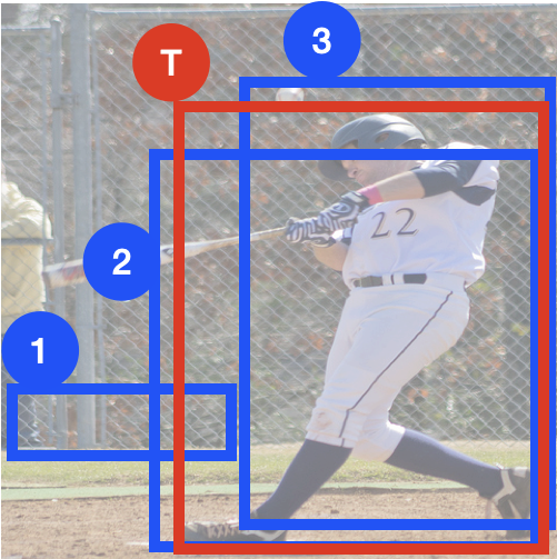
この直感を満たしてくれるのがIoUです.IoUは単純で下図のように,$IoU=\frac{オレンジ}{緑}$で定義されています.こうすれば重なりが大きいほど,値が大きくなり,直感に従いそうですね.
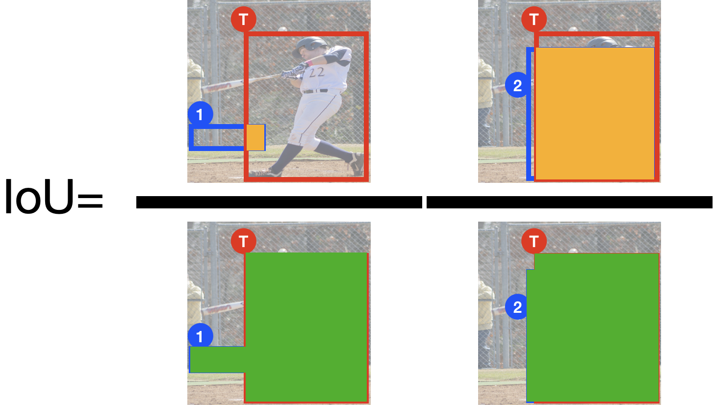
実際には,正解ラベルのバウンディングボックスと8732個全てのDefault BoxのIoU値を計算し,このIoUの閾値(0.5)を超えたDefault BoxにPersonクラスを付与,それ以外を背景(Background)クラスを付与します.
例:

Matching Strategyの実装
特にないですが,IoUの計算にはcentroids表記よりcorners表記の方が扱いやすいので,しっかり変換することに注意します.また,
# a's shape = (a_num, 1, 4), b's shape = (1, b_num, 4)
a, b = a.unsqueeze(1), b.unsqueeze(0)
で一気にブロードキャストで計算できるようにしています.
def matching_strategy(targets, dboxes, **kwargs):
    """
    :param targets: Tensor, shape is (batch*object num(batch), 1+4+class_labels)
    :param dboxes: shape is (default boxes num, 4)
    IMPORTANT: Note that means (cx, cy, w, h)
    :param kwargs:
        threshold: (Optional) float, threshold for returned indicator
        batch_num: (Required) int, batch size
    :return:
        pos_indicator: Bool Tensor, shape = (batch, default box num). this represents whether each default box is object or background.
        matched_targets: Tensor, shape = (batch, default box num, 4+class_num) including background
    """
    threshold = kwargs.pop('threshold', 0.5)
    batch_num = kwargs.pop('batch_num')
    device = dboxes.device


    dboxes_num = dboxes.shape[0]
    # minus 'box number per image' and 'localization=(cx, cy, w, h)'
    class_num = targets[0].shape[1] - 4

    # convert centered coordinated to minmax coordinates
    dboxes_mm = centroids2corners(dboxes)

    # create returned empty Tensor
    pos_indicator, matched_targets = torch.empty((batch_num, dboxes_num), device=device, dtype=torch.bool), torch.empty((batch_num, dboxes_num, 4 + class_num), device=device)

    # matching for each batch
    index = 0
    for b, target in enumerate(targets):
        targets_loc, targets_conf = target[:, :4], target[:, 4:]

        # overlaps' shape = (object num, default box num)
        overlaps = iou(centroids2corners(targets_loc), dboxes_mm.clone())

        # get maximum overlap value for each default box
        # shape = (batch num, dboxes num)
        overlaps_per_dbox, object_indices = overlaps.max(dim=0)
        #object_indices = object_indices.long() # for fancy indexing

        # get maximum overlap values for each object
        # shape = (batch num, object num)
        overlaps_per_object, dbox_indices = overlaps.max(dim=1)
        for obj_ind, dbox_ind in enumerate(dbox_indices):
            object_indices[dbox_ind] = obj_ind
        overlaps_per_dbox.index_fill_(0, dbox_indices, threshold + 1)# ensure N!=0

        pos_ind = overlaps_per_dbox > threshold

        # assign targets
        matched_targets[b, :, :4], matched_targets[b, :, 4:] = targets_loc[object_indices], targets_conf[object_indices]
        pos_indicator[b] = pos_ind

        # set background flag
        neg_ind = torch.logical_not(pos_ind)
        matched_targets[b, neg_ind, 4:] = 0
        matched_targets[b, neg_ind, -1] = 1


    return pos_indicator, matched_targets


def iou(a, b):
    """
    :param a: Box Tensor, shape is (nums, 4)
    :param b: Box Tensor, shape is (nums, 4)
    IMPORTANT: Note that 4 means (xmin, ymin, xmax, ymax)
    :return:
        iou: Tensor, shape is (a_num, b_num)
             formula is
             iou = intersection / union = intersection / (A + B - intersection)
    """

    # get intersection's xmin, ymin, xmax, ymax
    # xmin = max(a_xmin, b_xmin)
    # ymin = max(a_ymin, b_ymin)
    # xmax = min(a_xmax, b_xmax)
    # ymax = min(a_ymax, b_ymax)
    """
    >>> b
    tensor([2., 6.])
    >>> c
    tensor([1., 5.])
    >>> torch.cat((b.unsqueeze(1),c.unsqueeze(1)),1)
    tensor([[2., 1.],
            [6., 5.]])
    """
    # convert for broadcast
    # a's shape = (a_num, 1, 4), b's shape = (1, b_num, 4)
    a, b = a.unsqueeze(1), b.unsqueeze(0)
    intersection = torch.cat((torch.max(a[:, :, 0], b[:, :, 0]).unsqueeze(2),
                              torch.max(a[:, :, 1], b[:, :, 1]).unsqueeze(2),
                              torch.min(a[:, :, 2], b[:, :, 2]).unsqueeze(2),
                              torch.min(a[:, :, 3], b[:, :, 3]).unsqueeze(2)), dim=2)
    # get intersection's area
    # (w, h) = (xmax - xmin, ymax - ymin)
    intersection_w, intersection_h = intersection[:, :, 2] - intersection[:, :, 0], intersection[:, :, 3] - intersection[:, :, 1]
    # if intersection's width or height is negative, those will be converted to zero
    intersection_w, intersection_h = torch.clamp(intersection_w, min=0), torch.clamp(intersection_h, min=0)

    intersectionArea = intersection_w * intersection_h

    # get a and b's area
    # area = (xmax - xmin) * (ymax - ymin)
    A, B = (a[:, :, 2] - a[:, :, 0]) * (a[:, :, 3] - a[:, :, 1]), (b[:, :, 2] - b[:, :, 0]) * (b[:, :, 3] - b[:, :, 1])

    return intersectionArea / (A + B - intersectionArea)
正解ラベルの正規化!!
!!をつけているくらいなので,重要です!!
割り当てが完了したら,現論文の(2)式を使って,$i$番目のDefault Box$(d_i^{c_x},d_i^{c_y},d_i^{w},d_i^{h})$と正解ラベルのバウンディングボックス$(g_i^{c_x},g_i^{c_y},g_i^{w},g_i^{h})$のオフセット値$(\hat{g}_i^{c_x},\hat{g}_i^{c_y},\hat{g}_i^{w},\hat{g}_i^{h})$を求めます.
\begin{align}
(\hat{g}_i^{c_x},\hat{g}_i^{c_y}) &= \left( \frac{g_i^{c_x}-d_i^{c_x}}{d_i^{w}},\frac{g_i^{c_y}-d_i^{c_y}}{d_i^{h}} \right) \\
(\hat{g}_i^{w},\hat{g}_i^{h}) &= \left( \log{ \left( \frac{g_i^{w}}{d_i^{w}}\right)},\log{ \left( \frac{g_i^{h}}{d_i^{h}}\right)}\right) \tag{2}
\end{align}
ここまではいいのですが,実装の際には,もう1処理入ります.
僕が非常に参考にしたDeepに理解する深層学習による物体検出 by Keras
6: 5の値を予測したボックスの幅で割る(比率が分かる)
7: 6の値を予測したボックスの分散で割る
# dist b/t match center and prior's center
g_cxcy = (matched[:, :2] + matched[:, 2:])/2 - priors[:, :2]
# encode variance
g_cxcy /= (variances[0] * priors[:, 2:])
# match wh / prior wh
g_wh = (matched[:, 2:] - matched[:, :2]) / priors[:, 2:]
g_wh = torch.log(g_wh) / variances[1]
に見慣れぬ'variance'があります.このvariance(分散)で割る意味がどうしても理解できませんでした.初めはなんか確率的に予測するために必要なんだろって思っていて,この数値は無視していたのですが,何回学習させても収束しませんでした.めちゃくちゃ調べまくってようやく答えがBounding Box Encoding and Decoding in Object Detectionに見つかりました.
This variance input is extremely misleading.(中略)it is actually a process of standard normalization instead of “encoding with variance”.
どうやらこのvarianceは正規化処理らしいです.なるほど,正規化処理なら”variance”で割る理由もわかります.じゃあstdとした方が良さそうですね.さらには,mean=0と考えて,(2)式は最終的に
\begin{align*}
      (\hat{g}_{j}^{cx},\hat{g}_{j}^{cy})&=\left( \frac{\frac{g_{j}^{cx}-d_{i}^{cx}}{d_{i}^{w}}-\mu^{cx}}{\sigma^{cx}}, \frac{\frac{g_{j}^{cy}-d_{i}^{cy}}{d_{i}^{h}}-\mu^{cy}}{\sigma^{cy}} \right) \\
      (\hat{g}_{j}^{w}, \hat{g}_{j}^{h})&=\left( \frac{\log{\frac{g_j^{w}}{d_{i}^{w}}}-\mu^{w}}{\sigma^{w}}, \frac{\log{\frac{g_j^{h}}{d_{i}^{h}}}-\mu^{h}}{\sigma^{h}} \right)
  \end{align*} \tag{2'}
と書く方が良さそうです.この正規化処理をしたら,学習もサクサク進むようになりました.正規化って大事なんですね.
また,一般的に物体検出では,meanとstdの値は
$\bf{\mu}=(\mu^{cx},\mu^{cy},\mu^{w},\mu^{h})=(0,0,0,0),\bf{\sigma}=(\sigma^{cx},\sigma^{cy},\sigma^{w},\sigma^{h})=(0.1,0.1,0.2,0.2)$
を使うみたいです.
正解ラベルの正規化!!の実装
ここまでわかれば実装はそんなに難しくないです.このvariance問題にはだいぶ苦労させられたので,norm_stdsと強調してやりました笑
class Encoder(nn.Module):
    def __init__(self, norm_means=(0.0, 0.0, 0.0, 0.0), norm_stds=(0.1, 0.1, 0.2, 0.2)):
        super().__init__()

        norm_means = _check_norm('norm_means', norm_means)
        norm_stds = _check_norm('norm_stds', norm_stds)

        # shape = (1, 1, 4=(cx, cy, w, h)) or (1, 1, 1)
        self.norm_means = norm_means.unsqueeze(0).unsqueeze(0)
        self.norm_stds = norm_stds.unsqueeze(0).unsqueeze(0)


    def forward(self, targets, dboxes, batch_num):
        """
        :param targets: Tensor, shape is (batch*object num(batch), 1+4+class_labels)
        :param dboxes: Tensor, shape is (total_dbox_nums, 4=(cx,cy,w,h))
        :param batch_num: int
        :return:
            pos_indicator: Bool Tensor, shape = (batch, default box num). this represents whether each default box is object or background.
            encoded_boxes: Tensor, calculate ground truth value considering default boxes. The formula is below;
                           gt_cx = (gt_cx - dbox_cx)/dbox_w, gt_cy = (gt_cy - dbox_cy)/dbox_h,
                           gt_w = train(gt_w / dbox_w), gt_h = train(gt_h / dbox_h)
                           shape = (batch, default boxes num, 4)
        """
        # matching
        # pos_indicator: Bool Tensor, shape = (batch, default box num). this represents whether each default box is object or background.
        # targets: Tensor, shape = (batch, default box num, 4+class_num) including background
        pos_indicator, targets = matching_strategy(targets, dboxes, batch_num=batch_num)

        # encoding
        # targets_loc: Tensor, shape = (batch, default boxes num, 4)
        targets_loc = targets[:, :, :4]

        assert targets_loc.shape[1:] == dboxes.shape, "targets_loc and default_boxes must be same shape"

        gt_cx = (targets_loc[:, :, 0] - dboxes[:, 0]) / dboxes[:, 2]
        gt_cy = (targets_loc[:, :, 1] - dboxes[:, 1]) / dboxes[:, 3]
        gt_w = torch.log(targets_loc[:, :, 2] / dboxes[:, 2])
        gt_h = torch.log(targets_loc[:, :, 3] / dboxes[:, 3])

        encoded_boxes = torch.cat((gt_cx.unsqueeze(2),
                          gt_cy.unsqueeze(2),
                          gt_w.unsqueeze(2),
                          gt_h.unsqueeze(2)), dim=2)

        # normalization
        targets[:, :, :4] = (encoded_boxes - self.norm_means.to(targets_loc.device)) / self.norm_stds.to(targets_loc.device)

        return pos_indicator, targets
画像,正解ラベルを入力
↑で変換した正解ラベル,画像を使って,ようやく学習です.
順伝搬(L2Normalization)
基本的にモデル図(再再掲)に従って順伝搬させていくだけですが,1点だけ注意すべき点があります.
それは,Default Boxの作成で述べた「予測の大元となる特徴マップ」のConv4_3,Conv7,Conv8_2,Conv9_2,Conv10_2,Conv11_2のうち,小さい物体の情報を持つConv4_3のスケールが他と比べて違うので,正規化する点です.どうやら,入力側(図中左)のスケールは出力側(図中右)に比べると大きくなるらしいです.(ParseNetより)
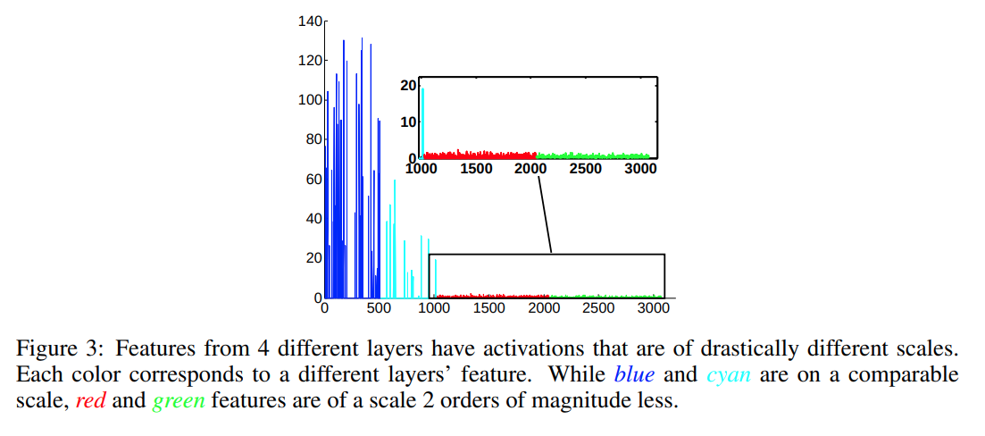
そのため,Conv4_3の出力を$\mathrm{x}_{c,j,i}$($c,j,i$はそれぞれチャンネル,高さ,幅)として,
\hat{\mathrm{x}}_{c,j,i}=\frac{\mathrm{x}_{c,j,i}}{\sqrt{\sum_d|x_{d,j,i}|^2}} \\
\hat{\mathrm{y}}_{c,j,i}=\gamma_{c}\hat{\mathrm{x}}_{c,j,i}
Channelの向きに対してL2距離を取ることで正規化します.ここで,$\gamma_{c}$をかける理由は,$\hat{\mathrm{x}}_{c,j,i}$の値が小さくなりすぎて学習が進まなくなることを防ぐためです.(ちなみにこの$\gamma_{c}$は定数ではなく変数です.初期値は10や20とするのが一般的らしく,SSDでは20を用います.)
※その関係から,SSD300では,Conv4_3ではスケールの式(1)に当てはめず,0.1を与えています.そのほかの層は,$s_{min}=0.2,s_{max}=0.9,m=5$としてスケールを計算します.
実装
PyTorchでは順伝搬の処理をtorch.nn.Moduleを継承したforward関数に記述します.上述のL2Normalizationは以下のように実装できます.
class L2Normalization(nn.Module):
    def __init__(self, channels, gamma=20):
        super().__init__()
        self.gamma = gamma
        self.in_channels = channels
        self.out_channels = channels
        self.scales = nn.Parameter(torch.Tensor(self.in_channels)) # trainable
        self.reset_parameters()

    def reset_parameters(self):
        init.constant_(self.scales, self.gamma) # initialized with gamma first

    # Note that pytorch's dimension order is batch_size, channels, height, width
    def forward(self, x):
        # |x|_2
        # normalize (x^)
        x = F.normalize(x, p=2, dim=1)
        return self.scales.unsqueeze(0).unsqueeze(2).unsqueeze(3) * x
SSDの順伝搬は以下のように実装しました.self.feature_layersにconv1_1~conv11_1をKeyに持つnn.ModuleDict,self.localization_layers,self.confidence_layersに図中のclassifierの畳み込みをKeyに持つnn.ModuleDict,self.addon_layersにL2NormalizationをKeyに持つnn.ModuleDictとして順伝搬させています.
class SSDBase(ObjectDetectionModelBase):

省略

    def forward(self, x):
        """
        :param x: Tensor, input Tensor whose shape is (batch, c, h, w)
        :return:
            predicts: localization and confidence Tensor, shape is (batch, total_dbox_num, 4+class_labels)
        """
        if not self.isBuilt:
            raise NotImplementedError(
                "Not initialized, implement \'build_feature\', \'build_classifier\', \'build_addon\'")

        # feature
        sources = []
        addon_i = 1
        for name, layer in self.feature_layers.items():
            x = layer(x)

            source = x
            if name in self.addon_source_names:
                if name not in self._train_config.classifier_source_names:
                    logging.warning("No meaning addon: {}".format(name))
                source = self.addon_layers['addon_{}'.format(addon_i)](source)
                addon_i += 1

            # get features by feature map convolution
            if name in self._train_config.classifier_source_names:
                sources += [source]

        # classifier
        locs, confs = [], []
        for source, loc_name, conf_name in zip(sources, self.localization_layers, self.confidence_layers):
            locs += [self.localization_layers[loc_name](source)]
            confs += [self.confidence_layers[conf_name](source)]

        predicts = self.predictor(locs, confs)
        return predicts

省略
Predictorでは,classifierの出力を(batch, total_dbox_num=8732, (4+class_labels))に変換しています.
class Predictor(nn.Module):
    def __init__(self, class_nums):
        super().__init__()

        self._class_nums = class_nums

    def forward(self, locs, confs):
        """
        :param locs: list of Tensor, Tensor's shape is (batch, c, h, w)
        :param confs: list of Tensor, Tensor's shape is (batch, c, h, w)
        :return: predicts: localization and confidence Tensor, shape is (batch, total_dbox_num * (4+class_labels))
        """
        locs_reshaped, confs_reshaped = [], []
        for loc, conf in zip(locs, confs):
            batch_num = loc.shape[0]

            # original feature => (batch, (class_num or 4)*dboxnum, fmap_h, fmap_w)
            # converted into (batch, fmap_h, fmap_w, (class_num or 4)*dboxnum)
            # contiguous means aligning stored 1-d memory for given array
            loc = loc.permute((0, 2, 3, 1)).contiguous()
            locs_reshaped += [loc.reshape((batch_num, -1))]

            conf = conf.permute((0, 2, 3, 1)).contiguous()
            confs_reshaped += [conf.reshape((batch_num, -1))]


        locs_reshaped = torch.cat(locs_reshaped, dim=1).reshape((batch_num, -1, 4))
        confs_reshaped = torch.cat(confs_reshaped, dim=1).reshape((batch_num, -1, self._class_nums))

        return torch.cat((locs_reshaped, confs_reshaped), dim=2)
localization lossとconfidence loss(hard negative mining)の計算
ロスの計算をする前に,もう一度何を予測するかを整理します.SSDが予測するのは,
- Default Boxとのオフセット値
- クラスラベル
です.「Default Boxとのオフセット値」≒「物体のバウンディングボックス」なので,位置(Localization)を予測しています.一方「クラスラベル」はその名の通り,クラスを予測しますが,その信頼度(Confidence)を予測しているともいえます.
なので,ロス計算ではこれらのLocalizationとConfidenceを正解に近づけるように別々に考えて計算し,最終的に一つのロスとします.
- Localizationロス
SmoothL1関数を使います.
L_{loc}(\mathbb{P},l,g)=\sum_{i\in \mathbb{P}}^N \sum_{m\in \{c_x,x_y,w,h\}} \mathrm{smoothL1}(l_i^m-\hat{g}_i^m)
ここで
- $l$:予測した「Default Boxとのオフセット値」
- $\mathbb{P}$:正解ラベルのバウンディングボックスをDefault Boxに割り当て(matching strategy)で背景でなくクラスラベルが割り当てられたDefault Boxの集合
です.
- Confidenceロス
LogSoftmax関数を使います.
L_{conf}(\mathbb{P},c)=-\sum_{p}\sum_{i\in \mathbb{P}}^N \log{(\hat{c}_i^p)}-\sum_{i\in \mathbb{B}^{hnm}}^{B^{hnm}} \log{(\hat{c}_i^b)} \\
\hat{c}_i^n = \frac{\exp{c_i^n}}{\sum_{n'} \exp{c_i^{n'}}}
ここで,$\mathbb{B}$は,$\mathbb{P}$の逆で背景と割り当てられたDefault Boxの集合です.ただし,このままでは$\mathbb{P}$に比べて$\mathbb{B}$の数が多くなってしまい,学習がうまく進みません.そこで,Hard negative miningを行います.Hard negative miningは,背景の信頼度$\hat{c}_i^b$を高い順にソートし,Negative:Positiveの比が$3:1=N:B^{hnm}$ になるようにすることです.
- 最終的なロス
L(\mathbb{P},c,l,g)=\frac{1}{N}(L_{conf}(\mathbb{P},c)+\alpha L_{loc}(\mathbb{P},l,g))
ここで,$N=|\mathbb{P}|$,$\alpha$は両者の重みです.(現論文では$\alpha=1$)
ロスの実装
実装は省略します.ここをみてください.
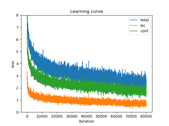
あとはPyTorchが自動で微分を行ってくれるので,収束するまで行えば良いです.
例:Voc2007+2012
おわりに
これも最後ガス欠しました.長すぎて最後まで読む方なんていないでしょうけど,どれかが参考になれば幸いです.
参考
- Default Box
- Encode and Decode
- Pretrained model
- mAP