
Qiita民が大好きなPythonで積のパーセプトロンを作成しました。
I created a perceptron of multiplication in Python which Qiita people love.
# coding=utf-8
import numpy as np
import matplotlib.pyplot as plt

# Initial value
# number of learning
N = 500
# layer
layer = [2, 2, 1]
# bias
# bias = [0.0, 0.0]
# learning rate
η = [1.0, 1.0]
# number of middle layers
H = len(η) - 1
# teacher value
mul = [None for _ in range(N)]
# function output value
f_out = [[None for _ in range(H + 1)] for _ in range(N)]
# function input value
f_in = [[None for _ in range(H + 1)] for _ in range(N)]
# weight
w = [[None for _ in range(H + 1)] for _ in range(N + 1)]
for h in range(H + 1):
    w[0][h] = np.random.uniform(-1, 1, (layer[h + 1], layer[h]))
print(w[0])
# squared error
dE = [None for _ in range(N)]
# ∂E/∂IN
δ = [[None for _ in range(H + 1)] for _ in range(N)]

# Learning
for n in range(N):

    #input value
    f_out[n][0] = np.random.uniform(-1, 1, ((layer[0]), 1))

    #teacher value
    mul[n] = f_out[n][0][0] * f_out[n][0][1]

    #order propagation
    f_in[n][0] = np.dot(w[n][0], f_out[n][0])
    f_out[n][1] = f_in[n][0] * f_in[n][0]

    #output value
    f_in[n][1] = np.dot(w[n][1], f_out[n][1])

    #squared error
    dE[n] = f_in[n][1] - mul[n]#value after squared error differentiation due to omission of calculation

    #back propagation
    δ[n][1] = 1.0 * dE[n]
    δ[n][0] = 2.0 * f_in[n][0] * w[n][1].T * δ[n][1]
    for h in range(H + 1):
        w[n + 1][h] = w[n][h] - η[h] * f_out[n][h].T * δ[n][h]

# Output
# Weight
print(w[N])

# figure
# area height
py = np.amax(layer)
# area width
px = (H + 1) * 2
# area size
plt.figure(figsize = (16, 9))
# horizontal axis
x = np.arange(0, N + 1, 1)
# drawing
for h in range(H + 1):
    for l in range(layer[h + 1]):
        #area matrix
        plt.subplot(py, px, px * l + h * 2 + 1)
        for m in range(layer[h]):
            #line
            plt.plot(x, np.array([w[n][h][l, m] for n in range(N + 1)]), label = "w[" + str(h) + "][" + str(l) + "," + str(m) + "]")
        #grid line
        plt.grid(True)
        #legend
        plt.legend(bbox_to_anchor = (1, 1), loc = 'upper left', borderaxespad = 0, fontsize = 10)

# save
plt.savefig('graph_mul.png')
# show
plt.show()
重みの考え方を示します。 \\
I\ indicate\ the\ concept\ of\ weight. \\
 \\
w[0]=
\begin{pmatrix}
△ & □\\
▲ & ■
\end{pmatrix}
,w[1]=
\begin{pmatrix}
○ & ●
\end{pmatrix}\\
 \\
入力値とw[0]の積 \\
multiplication\ of\ input\ value\ and\ w[0]\\
w[0]
\begin{pmatrix}
a\\
b
\end{pmatrix}
=
\begin{pmatrix}
△ & □\\
▲ & ■
\end{pmatrix}
\begin{pmatrix}
a\\
b
\end{pmatrix}
=
\begin{pmatrix}
△a + □b\\
▲a + ■b
\end{pmatrix}\\
 \\
第1層に入力\\
enter\ in\ the\ first\ layer\\
\begin{pmatrix}
(△a + □b)^2\\
(▲a + ■b)^2
\end{pmatrix}\\
 \\
第1層出力とw[1]の積=出力値\\
product\ of\ first\ layer\ output\ and\ w[1]\ =\ output\ value\\
\begin{align}
&
w[1]
\begin{pmatrix}
(△a + □b)^2\\
(▲a + ■b)^2
\end{pmatrix}\\
=&
\begin{pmatrix}
○ & ●
\end{pmatrix}
\begin{pmatrix}
(△a + □b)^2\\
(▲a + ■b)^2
\end{pmatrix}\\
=&〇(△a + □b)^2 + ●(▲a + ■b)^2\\
=&\quad (○△^2 + ●▲^2)a^2\\
&+(○□^2 + ●■^2)b^2\\\
&+(2〇△□+2●▲■)ab
\end{align}\\
 \\
なんだか、ややこしくなってしまってますが\\
とりあえずは、下記条件を満たせば積abを出力することができます。\\
It's\ getting\ confusing\\
For\ the\ moment,\ the\ multiplication\ ab\ can\ be\ output\ if\ the\ following\ conditions\ are\ satisfied.\\
\left\{
\begin{array}{l}
○△^2 + ●▲^2=0 \\
○□^2 + ●■^2=0 \\
2〇△□+2●▲■=1
\end{array}
\right.
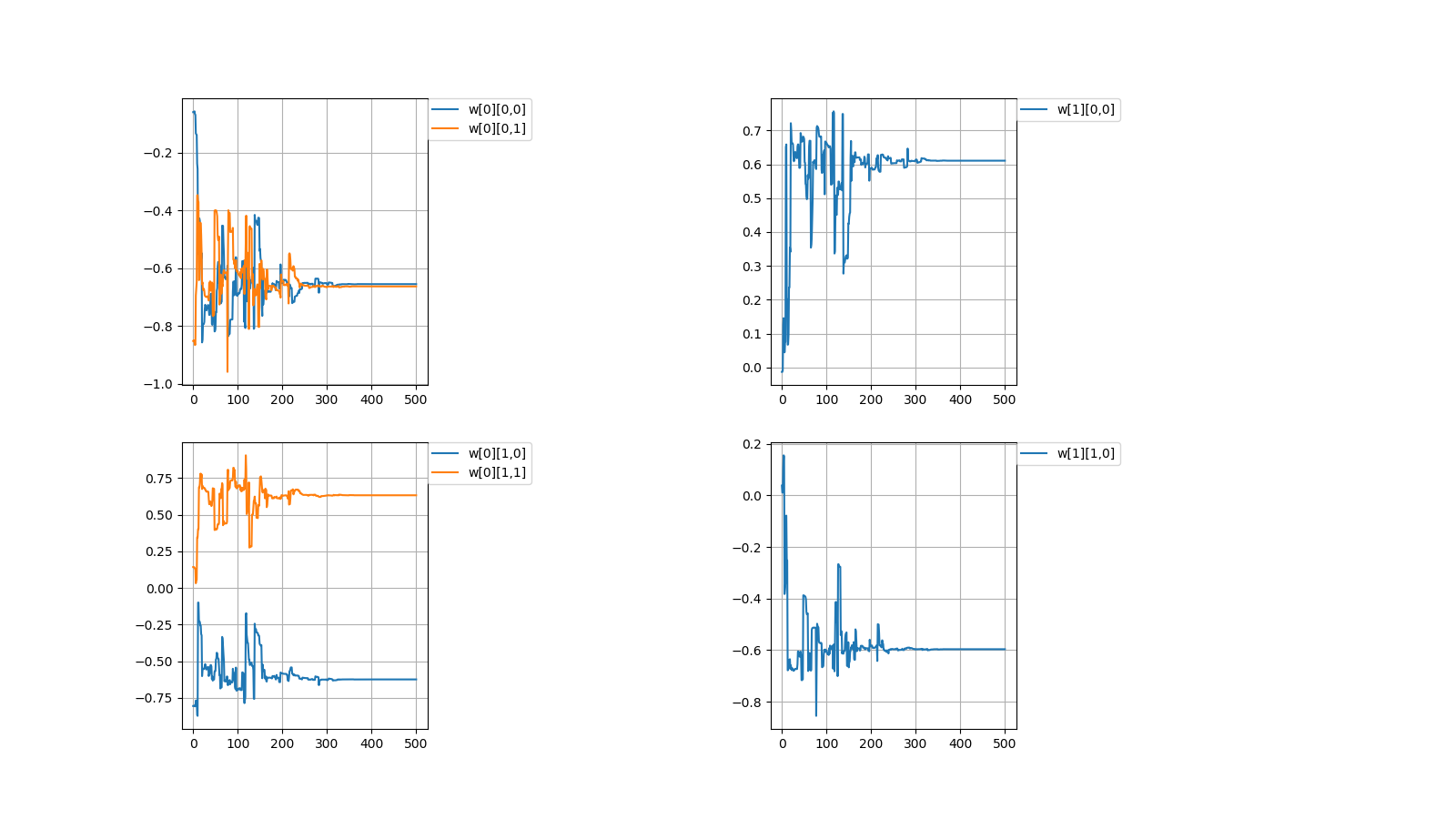
毎度恒例、初期値を乱数(-1.0~1.0)で決めてから学習を繰り返すと目標値に収束するか試してみました。
After deciding the initial value between random numbers (-1.0~1.0),
I tried to repeat the learning to converge to the target value.
目標値\\
Target\ value\\
w[0]=
\begin{pmatrix}
△ & □\\
▲ & ■
\end{pmatrix}
,w[1]=
\begin{pmatrix}
○ & ●
\end{pmatrix}\\
\left\{
\begin{array}{l}
○△^2 + ●▲^2=0 \\
○□^2 + ●■^2=0 \\
2〇△□+2●▲■=1
\end{array}
\right.\\
 \\
初期値\\
Initial\ value\\
w[0]=
\begin{pmatrix}
-0.06001642 & -0.80560397\\
-0.85252436 & 0.14216594
\end{pmatrix}
,w[1]=
\begin{pmatrix}
-0.01316071 & 0.03798114
\end{pmatrix}\\
\left\{
\begin{array}{l}
○△^2 + ●▲^2=0.0275572039 \\
○□^2 + ●■^2=-0.0077736286 \\
2〇△□+2●▲■=-0.0104792494
\end{array}
\right.\\
 \\
計算値\\
Calculated\ value\\
w[0]=
\begin{pmatrix}
-0.65548785 & -0.62435684\\
-0.66341526 & 0.63186139
\end{pmatrix}
,w[1]=
\begin{pmatrix}
0.61080948 & -0.59638741
\end{pmatrix}\\
\left\{
\begin{array}{l}
○△^2 + ●▲^2=-3.88711177092826E-5 \\
○□^2 + ●■^2=-3.21915003292927E-7 \\
2〇△□+2●▲■=0.9999528147
\end{array}
\right.
成功しましたが課題を抱えています。
It was successful but with challenges.
1,収束する時と収束しない時がある
1,There are cases when it converges and when it doesn't converge
初期値\\
Initial\ value\\
w[0]=
\begin{pmatrix}
0.96898039 & 0.5250381\\
-0.13805777 & -0.457846
\end{pmatrix}
,w[1]=
\begin{pmatrix}
0.17181768 & 0.27522847
\end{pmatrix}\\

計算値\\
Calculated\ value\\
w[0]=
\begin{pmatrix}
0.37373305 & 0.53163593\\
-0.38455151 & -0.54773647
\end{pmatrix}
,w[1]=
\begin{pmatrix}
0.34178043 & 0.33940928
\end{pmatrix}\\
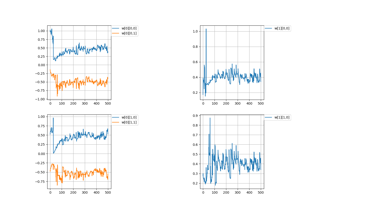
上記のように値が収束しない場合がときたまあります。
本当はプログラムを組んで収束しない時の統計を出すべきなんでしょうが
そこまでの気力がありませんでした。
Occasionally, the values don't converge as described above.
Properly, it should be put out the statistics when doesn't converge by programming
I didn't have the energy to get it.
2,収束したらしたでいつも同じぐらいの値で収束する
どういう訳か、例えばw[0][0,0]=±0.6...ぐらいの値に落ち着く事がほとんどです。
2,It always converges with the similar value
For some reason, for example, it is almost always settled to the value of w[0][0,0]=±0.6...
一見、簡単そうなパーセプトロンでも謎が多いです。
At first glance, even the seemingly easy perceptron has many mystery.
NEXT【/】