
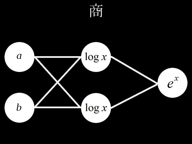
深層学習の形式でわり算のパーセプトロンを考えてみました。
I considered a division perceptron in the form of deep learning.
# coding=utf-8
import numpy as np
import matplotlib.pyplot as plt

# Initial value
# number of learning
N = 1000
# layer
layer = [2, 2, 1]
# bias
# bias = [0.0, 0.0]
# learning rate
η = [0.001, 0.001]
# η = [0.000001, 0.000001]
# number of middle layers
H = len(η) - 1
# teacher value
t = [None for _ in range(N)]
# function output value
f_out = [[None for _ in range(H + 1)] for _ in range(N)]
# function input value
f_in = [[None for _ in range(H + 1)] for _ in range(N)]
# weight
w = [[None for _ in range(H + 1)] for _ in range(N + 1)]
for h in range(H + 1):
    w[0][h] = np.random.uniform(-1.0, 1.0, (layer[h + 1], layer[h]))

for h in range(H + 1):
    print(w[0][h])

# squared error
dE = [None for _ in range(N)]
# ∂E/∂IN
δ = [[None for _ in range(H + 1)] for _ in range(N)]

# Learning
for n in range(N):

    #input value
    f_out[n][0] = np.random.uniform(-10.0, 10.0, (layer[0]))

    #teacher value
    t[n] = f_out[n][0][0] / f_out[n][0][1]

    #order propagation
    f_in[n][0] = np.dot(w[n][0], f_out[n][0])
    f_out[n][1] = np.log(f_in[n][0]*f_in[n][0])
    f_in[n][1] = np.dot(w[n][1], f_out[n][1])

    #output value
    div = np.exp(f_in[n][1])

    #squared error
    dE[n] = div - t[n]#value after squared error differentiation due to omission of calculation

    #δ
    δ[n][1] = div * dE[n]
    δ[n][0] = (2.0 / f_in[n][0]) * np.dot(w[n][1].T, δ[n][1])

    #back propagation
    for h in range(H + 1):
        w[n + 1][h] = w[n][h] - η[h] * np.real(δ[n][h].reshape(len(δ[n][h]), 1) * f_out[n][h])


# Output
# Weight
for h in range(H + 1):
    print(w[N][h])
# figure
# area height
py = np.amax(layer)
# area width
px = (H + 1) * 2
# area size
plt.figure(figsize = (16, 9))
# horizontal axis
x = np.arange(0, N + 1, 1)
# drawing
for h in range(H + 1):
    for l in range(layer[h + 1]):
        #area matrix
        plt.subplot(py, px, px * l + h * 2 + 1)
        for m in range(layer[h]):
            #line
            plt.plot(x, np.array([w[n][h][l, m] for n in range(N + 1)]), label = "w[" + str(h) + "][" + str(l) + "," + str(m) + "]")
        #grid line
        plt.grid(True)
        #legend
        plt.legend(bbox_to_anchor = (1, 1), loc = 'upper left', borderaxespad = 0, fontsize = 10)

# save
plt.savefig('graph_div.png')
# show
plt.show()
重みの考え方を示します。\\
I\ indicate\ the\ concept\ of\ weight.\\
w[0]=
\begin{pmatrix}
△ & □\\
▲ & ■
\end{pmatrix},
w[1]=
\begin{pmatrix}
〇 & ●
\end{pmatrix}\\
 \\
入力値とw[0]の積\\
multiplication\ of\ input\ value\ and\ w[0]\\
\begin{pmatrix}
△ & □\\
▲ & ■
\end{pmatrix}
\begin{pmatrix}
a\\
b
\end{pmatrix}\\
=
\begin{pmatrix}
△a+□b\\
▲a+■b
\end{pmatrix}\\
 \\
第1層入力\\
enter\ in\ the\ first\ layer\\
\begin{pmatrix}
log(△a+□b)^2\\
log(▲a+■b)^2
\end{pmatrix}\\
 \\
負の数に対応するため真数を2乗しています。\\
The\ exact\ number\ is\ squared\ to\ accommodate\ negative\ numbers.\\
 \\
第1層出力とw[1]の積\\
product\ of\ first\ layer\ output\ and\ w[1]\\
\begin{align}
\begin{pmatrix}
〇 & ●
\end{pmatrix}
\begin{pmatrix}
log(△a+□b)^2\\
log(▲a+■b)^2
\end{pmatrix}
=&〇log(△a+□b)^2+●log(▲a+■b)^2\\
=&log(△a+□b)^{2〇}-log(▲a+■b)^{-2●}\\
=&log\frac{(△a+□b)^{2〇}}{(▲a+■b)^{-2●}}\\
\end{align}\\
 \\
出力層入力\\
enter\ in\ the\ output\ layer\\
e^{log\frac{(△a+□b)^{2〇}}{(▲a+■b)^{-2●}}}=\frac{(△a+□b)^{2〇}}{(▲a+■b)^{-2●}}\\
 \\
\left\{
\begin{array}{l}
△=1,□=0,〇=0.5 \\
▲=0,■=1,●=-0.5
\end{array}
\right.\\
 \\
\frac{a}{b}\\
 \\
最も簡単な場合、上記、条件を満たせば商a/bを出力することができます。\\
In\ the\ simplest\ case,\ if\ the\ above\ conditions\ are\ met,\ quotient\ a/b\ can\ be\ output.\\
初期値を乱数(-1.0~1.0)で決めてから学習を繰り返すと目標値に収束するか試してみました。\\
After\ deciding\ the\ initial\ value\ between\ random\ numbers\ (-1.0~1.0),\\
I\ tried\ to\ repeat\ the\ learning\ to\ converge\ to\ the\ target\ value.\\
 \\
目標値\\
Target\ value\\
w[0]=
\begin{pmatrix}
△ & □\\
▲ & ■
\end{pmatrix}
,w[1]=
\begin{pmatrix}
○ & ●
\end{pmatrix}\\
\left\{
\begin{array}{l}
△=1,□=0,〇=0.5 \\
▲=0,■=1,●=-0.5
\end{array}
\right.\\
 \\
初期値\\
Initial\ value\\
w[0]=
\begin{pmatrix}
-0.18845444 & -0.56031414\\
-0.48188658 & 0.6470921
\end{pmatrix}
,w[1]=
\begin{pmatrix}
0.80395641 & 0.80365676
\end{pmatrix}\\
\left\{
\begin{array}{l}
△=-0.18845444,□=-0.56031414,〇=0.80395641 \\
▲=-0.48188658,■=0.6470921,●=0.80365676
\end{array}
\right.\\
 \\
計算値\\
Calculated\ value\\
w[0]=
\begin{pmatrix}
14601870.60282903 & -14866110.02378938\\
13556781.27758209 & -13802110.45958244
\end{pmatrix}
,w[1]=
\begin{pmatrix}
-1522732.53915774 & -6080851.59710287
\end{pmatrix}\\
\left\{
\begin{array}{l}
△=14601870.60282903,□=-14866110.02378938,〇=-1522732.53915774 \\
▲=13556781.27758209,■=-13802110.45958244,●=-6080851.59710287
\end{array}
\right.\\
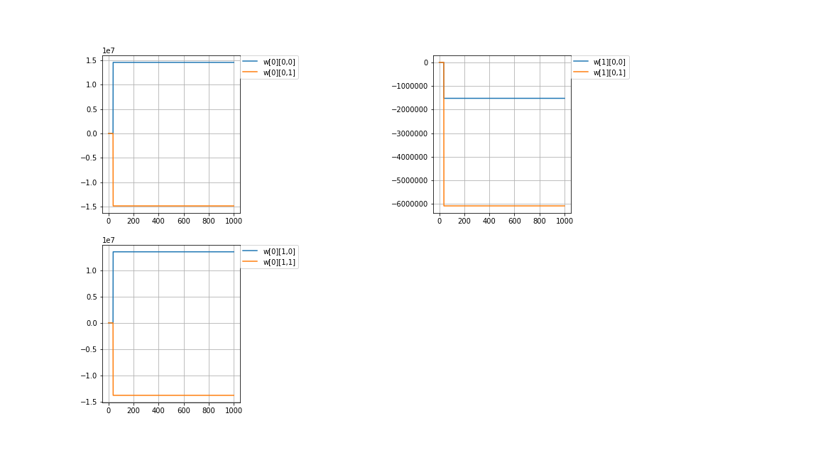
失敗です。何回やっても、重みがとんでもない値に発散してしまいます。\\
原因を探りました。\\
It\ is\ a\ failure.\\
No\ matter\ how\ many\ times\ I\ do,\ the\ weights\ will\ diverge\ to\ ridiculous\ values.\\
I\ investigated\ the\ cause.\\
 \\
誤差逆伝播の連鎖律で\\
In\ chain\ rule\ of\ the\ backpropagation\\
(log(x^2))'=\frac{2}{x}\\
\lim_{x \to ±∞} \frac{2}{x}=0\\
 \\
(e^x)'=e^x\\
\lim_{x \to -∞} e^x=0\\
このように極端に大きい値を取って、勾配消失させてしまうことがわかりました。\\
It\ was\ found\ that\ such\ an\ extremely\ large\ value\ would\ cause\ the\ gradient\ to\ disappear.\\
 \\
考え直しました。\\
I reconsidered.
# coding=utf-8
import numpy as np
import matplotlib.pyplot as plt

# Initial value
# number of learning
N = 200000
# layer
layer = [2, 2, 1]
# bias
# bias = [0.0, 0.0]
# learning rate
η = [0.1, 0.1]
# η = [0.000001, 0.000001]
# clip value
# clip = 709
clip = 700
# number of middle layers
H = len(η) - 1
# teacher value
t = [None for _ in range(N)]
# function output value
f_out = [[None for _ in range(H + 1)] for _ in range(N)]
# function input value
f_in = [[None for _ in range(H + 1)] for _ in range(N)]
# weight
w = [[None for _ in range(H + 1)] for _ in range(N + 1)]
for h in range(H):
    w[0][h] = np.random.uniform(-1.0, 1.0, (layer[h + 1], layer[h]))
w[0][H] = np.zeros((layer[H + 1], layer[H]))

for h in range(H + 1):
    print(w[0][h])

# squared error
dE = [None for _ in range(N)]
# ∂E/∂IN
δ = [[None for _ in range(H + 1)] for _ in range(N)]

# Learning
for n in range(N):

    #input value
    t[n] = clip
    while np.abs(t[n]) > np.log(np.log(clip)):#Gradient vanishing problem Measure
        f_out[n][0] = np.random.uniform(0.0, 10.0, (layer[0]))
        f_out[n][0] = np.array(f_out[n][0], dtype=np.complex)

        #teacher value
        t[n] = f_out[n][0][0] / f_out[n][0][1]

    #order propagation
    f_in[n][0] = np.dot(w[n][0], f_out[n][0])
    f_out[n][1] = np.log(f_in[n][0])
    f_in[n][1] = np.dot(w[n][1], f_out[n][1])

    #output value
    div = np.exp(f_in[n][1])

    #squared error
    dE[n] = np.real(div - t[n])#value after squared error differentiation due to omission of calculation
    dE[n] = np.clip(dE[n], -clip, clip)
    dE[n] = np.nan_to_num(dE[n])

    #δ
    δ[n][1] = np.real(div * dE[n])
    δ[n][1] = np.clip(δ[n][1], -clip, clip)
    δ[n][1] = np.nan_to_num(δ[n][1])


    δ[n][0] = np.real((1.0 / f_in[n][0]) * np.dot(w[n][1].T, δ[n][1]))
    δ[n][0] = np.clip(δ[n][0], -clip, clip)
    δ[n][0] = np.nan_to_num(δ[n][0])

    #back propagation
    for h in range(H + 1):
        #Gradient vanishing problem Measure
        # a*10^b a part only
        w10_u = np.real(δ[n][h].reshape(len(δ[n][h]), 1) * f_out[n][h])
        w10_u = np.clip(w10_u, -clip, clip)
        w10_u = np.nan_to_num(w10_u)
        w10_d = np.where(
            w10_u != 0.0,
            np.modf(np.log10(np.abs(w10_u)))[1],
            0.0
        )
        #Decimal not supported
        w10_d = np.clip(w10_d, 0.0, clip)

        w[n + 1][h] = w[n][h] - η[h] * (w10_u / np.power(10.0, w10_d))

# Output
# Weight
for h in range(H + 1):
    print(w[N][h])
# figure
# area height
py = np.amax(layer)
# area width
px = (H + 1) * 2
# area size
plt.figure(figsize = (16, 9))
# horizontal axis
x = np.arange(0, N + 1, 1) #0からN+1まで1刻み
# drawing
for h in range(H + 1):
    for l in range(layer[h + 1]):
        #area matrix
        plt.subplot(py, px, px * l + h * 2 + 1)
        for m in range(layer[h]):
            #line
            plt.plot(x, np.array([w[n][h][l, m] for n in range(N + 1)]), label = "w[" + str(h) + "][" + str(l) + "," + str(m) + "]")
        #grid line
        plt.grid(True)
        #legend
        plt.legend(bbox_to_anchor = (1, 1), loc = 'upper left', borderaxespad = 0, fontsize = 10)

# save
plt.savefig('graph_div.png')
# show
plt.show()
対策として
・入力値を複素数にする。
・教師値でオーバーフローしにくいデータだけにする。
・δを一定以上の大きな値にしない。
・勾配を a10^b のa部分だけにして重みが発散しないようにする。(bが正の数の時だけ)
As a countermeasure
・ Change the input value to a complex number.
・ Use only data that is difficult to overflow with the teacher value.
・ Do not make δ larger than a certain value.
・ Set the gradient to only a part of a10^b so that the weight does not diverge. (Only when b is a positive number)
目標値\\
Target\ value\\
w[0]=
\begin{pmatrix}
△ & □\\
▲ & ■
\end{pmatrix}
,w[1]=
\begin{pmatrix}
○ & ●
\end{pmatrix}\\
\left\{
\begin{array}{l}
△=1,□=0,〇=1 \\
▲=0,■=1,●=-1
\end{array}
\right.\\
\\
初期値\\
Initial value\\
w[0]=
\begin{pmatrix}
-0.12716087 & 0.34977234\\
0.85436489 & 0.65970844
\end{pmatrix}
,w[1]=
\begin{pmatrix}
0.0 & 0.0
\end{pmatrix}\\
\left\{
\begin{array}{l}
△=-0.12716087,□=0.34977234,〇=0.0 \\
▲=0.85436489,■=0.65970844,●=0.0
\end{array}
\right.\\
\\
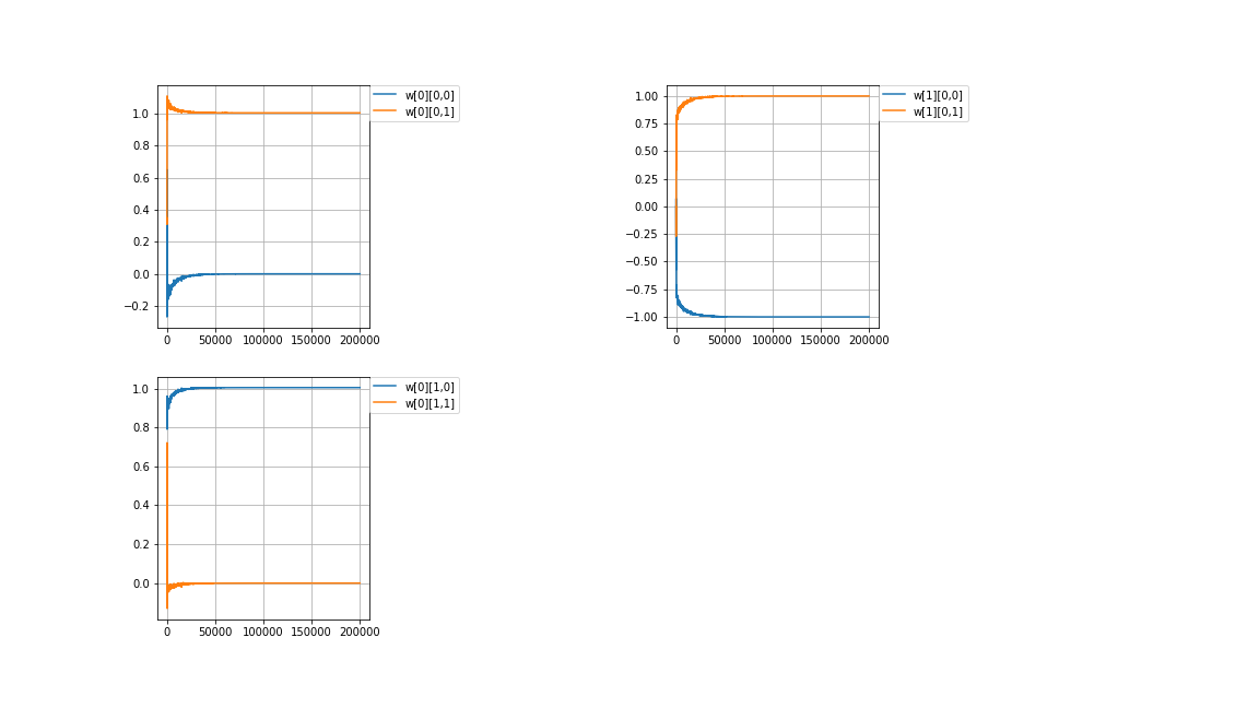
計算値\\
Calculated\ value\\
w[0]=
\begin{pmatrix}
-1.71228449e-08 & 1.00525062e+00\\
1.00525061e+00 & -4.72288257e-09
\end{pmatrix}
,w[1]=
\begin{pmatrix}
-0.99999998 & 0.99999998
\end{pmatrix}\\
\left\{
\begin{array}{l}
△=-1.71228449e-08,□=1.00525062e+00,〇=-0.99999998\\
▲=1.00525061e+00,■=-4.72288257e-09,●=0.99999998
\end{array}
\right.\\
\\
成功しました。△□と▲■の値が逆になっています。\\
正解ありきでそれに寄せていってるようなやり方で大分、気に入らないです。\\
それにしても、たかだか割り算を教えようとする程度でlog,exp,複素数と\\
高校数学まで拡張しなきゃいけないとは困ったもんです。\\
\\
Succeeded.\ The\ values\ of\ △□\ and\ ▲■\ are\ reversed.\\
I\ don't\ like\ it\ in\ the\ way\ that\ I\ get\ it\ right.\\
Even\ so,\ at\ the\ very\ least\ trying\ to\ teach\ division\\
log,\ exp,\ complex\ numbers\\
I\ had\ trouble\ expanding\ to\ high\ school\ mathematics.\\