Tabular Playground Series - Jun 2021- Day2

はじめに

　前回のDay1では自分ができたことを中心に書いたのでDay2ではKagglerの人達が行ってきたデータ分析を模倣しようと思います。特に今回はモデル構築ではなくデータの可視化を中心に取り扱います。モデル構築についてはDay3で取り扱う予定です。

以下参考にしたKaggler様の記事を載せておきます。
TPS June 2021 EDA
TPS May 2021 EDA & Model
[TPS-Jun] This is Original EDA & VIZ
⚡Catboost with Optuna Starter [TPS-06]

前回の記事で取り扱わなかったことを中心に(大半ですが)取り扱うので、コード等は最小限にとどめておきます。どうしても普遍性のある記事にはならないと思いますがあらかじめご了承ください。また、統率のとれてない目次にも目をつぶっていただけると助かります。

本文中にでてくる用語説明だけ軽く...
・目標変数(目的変数) = target = Class1~9
・説明変数 = features(計75個) = 特徴
・特徴量 = 説明変数の中の値

TPS June 2021EDA

参考:TPS June 2021 EDA

データの読み込み

## import packages
import os
import joblib    #並列化、直列化、メモ化など便利な機能を寄せ集めたようなPythonライブラリ
import numpy as np
import pandas as pd
import warnings

import matplotlib
import matplotlib.pyplot as plt
from matplotlib import ticker
import seaborn as sns

## setting up options
pd.set_option('display.max_rows', None)
pd.set_option('display.max_columns', None)
warnings.filterwarnings('ignore')

## import datasets
train_df = pd.read_csv('train.csv')
test_df = pd.read_csv('test.csv')
submission = pd.read_csv('sample_submission.csv')

実行に影響のない警告を非表示に

import warnings
warnings.filterwarnings('ignore')

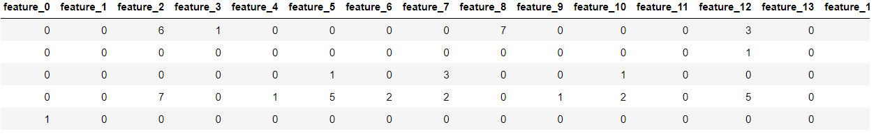
一応データの形式はつぎのようになっています
Day1の記事読んでない方は読んだ方がもしかするといいかもしれません。
Day1

train_df.head()

列と行、欠損値の有無を表示

print(f'Number of rows: {train_df.shape[0]};  Number of columns: {train_df.shape[1]}; No of missing values: {sum(train_df.isna().sum())}')

記事の方ではテストデータセットと提出用データセットについてもデータの分析を行っていました。例えば、データが所属する確率がtrainデータセットとtestデータセット、提出用データセットで同じ確率分布をもっていれば、モデル構築がそうでない場合より簡単になる(=同じデータセットを分割してそれぞれ3つのデータセットに分割している。)みたいな感じです。

データの分析

・モデルに使える特徴量の個数は75個
・それぞれの特徴量でユニークな値(特異な値、unique value)を見渡す
　→データの分布をみる
・それぞれの特徴量について訓練データセットとテストデータセットを比較する

データを可視化するときに必要な前処理

今回のデータの可視化では、データごとの特徴量の分布に応じたものを行うため、それに準じた前処理を行っています。そのため、基本的に特徴量に現れるユニークな値の個数を扱いやすいように加工してます。

# featuresのリスト
# カラムの中でidとtargetが含まれない列(=feature列)をリスト形式で取得
features = [feature for feature in train_df.columns if feature not in ['id', 'target']]

unique_values_train = np.zeros(2) # 2×1の0だけのリスト
for feature in features: # すべてのfeatureに対して
    temp = train_df[feature].unique() # temp = あるfeatureに含まれる数字の種類
    unique_values_train = np.concatenate([unique_values_train, temp])
    # [0 0 temp.... ] っていう感じになる
# 最初の00以外のリスト    
unique_values_train = np.unique(unique_values_train)

# テストデータセットについても同じ処理を
unique_values_test = np.zeros(2)
for feature in features:
    temp = test_df[feature].unique()
    unique_values_test = np.concatenate([unique_values_test, temp])
unique_values_test = np.unique(unique_values_test)

unique_value_feature_train = pd.DataFrame(train_df[features].nunique()) # ユニークな数の種類の数を羅列する
unique_value_feature_train = unique_value_feature_train.reset_index(drop=False) # インデックスを割り振って
unique_value_feature_train.columns = ['Features', 'Count'] # カラムを設定して新しくデータフレームを作っている
unique_value_feature_test = pd.DataFrame(test_df[features].nunique())
unique_value_feature_test = unique_value_feature_test.reset_index(drop=False)
unique_value_feature_test.columns = ['Features', 'Count']

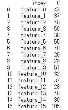
unique_value_feature_trainは次のような形式になります。各特長量とそれに付随するユニークな数の種類の個数がわかります。

次に、この訓練データとテストデータのユニークな数の種類のデータをもとに、特徴量の種類に違いがあるか確認します。

unique_value_feature_diff = unique_value_feature_train.copy()
# trainデータとtestデータで現れる特徴量の種類に違いがあるかどうか
unique_value_feature_diff['Count'] = unique_value_feature_train['Count'] - unique_value_feature_test['Count']
unique_value_feature_diff = unique_value_feature_diff[unique_value_feature_diff['Count']!=0]
print(unique_value_feature_diff) # 差分が0じゃない特徴をリストアップ

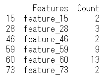
例えば、feature_15は訓練データセットの方がテストデータセットよりも2個多くユニークな特徴量が含まれていることになります。一方でこのデータに含まれないデータについては、訓練データとテストデータのユニークな特徴量が等しいことになります。ただし、訓練データとテストデータのユニークな特徴量が全て等しいということは保証できません。

transpose_features_train = train_df[features]
# 行ごとにpd.Series.value_counts(データの値の頻度を計算する関数)を適用させ、値が入ってない箇所を0で埋める
transpose_features_train = transpose_features_train.apply(pd.Series.value_counts, axis=1).fillna(0)
transpose_features_test = test_df[features]
transpose_features_test = transpose_features_test.apply(pd.Series.value_counts, axis=1).fillna(0)

transpose_features_trainの詳細

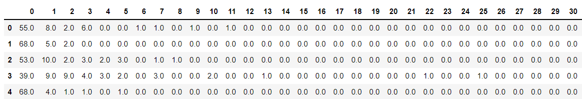
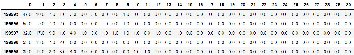
各データごとに特徴量が0、1、...の個数をそれぞれカウントした感じです。生のデータ見るとどういうコードなのかわかるかもしれない...

データの可視化

先ほど、訓練データとテストデータのユニークな特徴量が全て等しいということは保証できません的なことを言ってたので、それを裏付けるために出現する特徴量を可視化します。主に棒グラフ(横向き)を使い、訓練データセットとデータセットがそれぞれ同じ確率分布に従っているか、またはそうでないかを判断することができます。

データの範囲

plt.rcParams['figure.dpi'] = 600  # 図の解像度をあがる、横幅(縦幅)×dpiで決まるらしい
fig = plt.figure(figsize=(5, 0.8), facecolor='#f6f5f5') #図の大きさと背景色を変える
gs = fig.add_gridspec(2, 1) # 図をnrows, ncolsに分割する。2:1なので上下2分割
gs.update(wspace=0.4, hspace=0.8) # 図の同士の横、縦の間隔

background_color = "#f6f5f5"
sns.set_palette(['#ffd514']) # 図に使うカラーパレット

ax0 = fig.add_subplot(gs[0, 0]) # 2分割したうちの0行目0列目に図を描画する
for s in ["right", "top", "left"]: # グラフの右軸、上軸、左軸の線を見えなくする
    ax0.spines[s].set_visible(False)
ax0.set_facecolor(background_color) # 背景色の設定
ax0.tick_params(axis = "y", which = "both", left = False) # 縦軸、横軸の目盛設定
ax0_sns = sns.histplot(ax=ax0, x=unique_values_train, zorder=2, bins=352, linewidth=0, alpha=1)
ax0_sns.set_xlabel("Unique values",fontsize=4, weight='bold')
ax0_sns.tick_params(labelsize=4, width=0.5, length=1.5) #ラベルの際をの設定
ax0_sns.get_yaxis().set_visible(False) # 縦軸を見えなくする
ax0.text(-18, 2.3, 'Unique Values', fontsize=6, ha='left', va='top', weight='bold') # 左上のテキスト
ax0.text(-18, 1.9, 'Unique value for train and test dataset', fontsize=4, ha='left', va='top')
ax0_sns.legend(['Train', 'Test'], ncol=2, facecolor=background_color, edgecolor=background_color, fontsize=3, bbox_to_anchor=(-0.01, 1.6), loc='upper left') # 凡例の設定

background_color = "#f6f5f5"
sns.set_palette(['#ff355d'])

ax1 = fig.add_subplot(gs[1, 0])
for s in ["right", "top", "left"]:
    ax1.spines[s].set_visible(False)
ax1.set_facecolor(background_color)
ax1.tick_params(axis = "y", which = "both", left = False)
ax1_sns = sns.histplot(ax=ax1, x=unique_values_test, zorder=2, bins=352, linewidth=0, alpha=1)
ax1_sns.set_xlabel("Unique values",fontsize=4, weight='bold')
ax1_sns.tick_params(labelsize=4, width=0.5, length=1.5)
ax1_sns.get_yaxis().set_visible(False)
ax1_sns.legend(['Test'], ncol=2, facecolor=background_color, edgecolor=background_color, fontsize=3, bbox_to_anchor=(0.06, 3.4), loc='upper left')

plt.show()

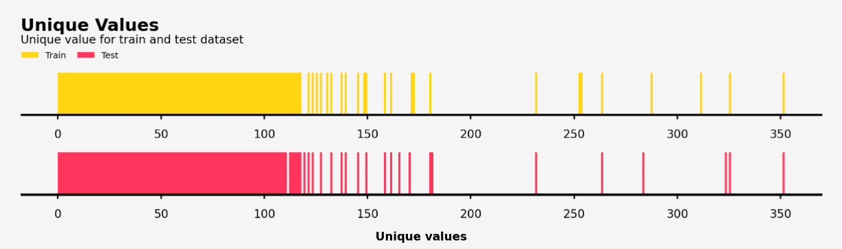
【可視化結果】
・ユニークな特徴量の値は0~100をこえて300近くまで散布している(0~352)
・ほぼほぼ似たような分布をとっている。

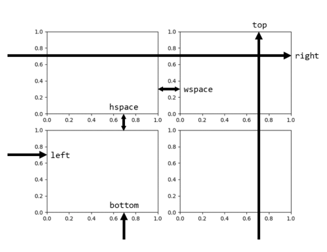
図の幅の引数

matplotlibの引数でよくでてくるleft, bottom, hspace...は以下の図にわかりやすく書いてありました。
matplotlibのグラフの箱の大きさを正確に把握したかった

カラーパレット

例えば以下のように検索すると(Googleで)カラーパレットが表示されます。このカラーパレットのHEXに対応する値をsns.set_paletteで設定できます。

各特徴量でのユニークな値の分布の可視化

plt.rcParams['figure.dpi'] = 600
fig = plt.figure(figsize=(4, 12), facecolor='#f6f5f5')
gs = fig.add_gridspec(1, 2)
gs.update(wspace=0.4, hspace=0.1)

background_color = "#f6f5f5"
sns.set_palette(['#ffd514']*75)

ax0 = fig.add_subplot(gs[0, 0])
for s in ["right", "top"]:
    ax0.spines[s].set_visible(False)
ax0.set_facecolor(background_color)
ax0_sns = sns.barplot(ax=ax0, y=unique_value_feature_train['Features'], x=unique_value_feature_train['Count'], 
                      zorder=2, linewidth=0, orient='h', saturation=1, alpha=1)
ax0_sns.set_xlabel("Unique Values",fontsize=4, weight='bold')
ax0_sns.set_ylabel("Features",fontsize=4, weight='bold')
ax0_sns.tick_params(labelsize=4, width=0.5, length=1.5)
ax0_sns.grid(which='major', axis='x', zorder=0, color='#EEEEEE', linewidth=0.4)  # 格子線(グリッド線)の表示
ax0_sns.grid(which='major', axis='y', zorder=0, color='#EEEEEE', linewidth=0.4)
ax0.text(0, -1.9, 'Unique Values - Train Dataset', fontsize=6, ha='left', va='top', weight='bold')
ax0.text(0, -1.2, 'feature_15 has the highest unique value', fontsize=4, ha='left', va='top')
# data label
# ax0に格納されている棒グラフをax0.patchesで取り出し、それの情報に基づいて棒グラフの隣にラベルを表示する
# p=0は右のようなものになっている   Rectangle(xy=(0, -0.4), width=42, height=0.8, angle=0)
for p in ax0.patches:
    value = f'{p.get_width():.0f}'
    x = p.get_x() + p.get_width() + 7 #  = 0 + 42 +7 = 49となる
    y = p.get_y() + p.get_height() / 2 
    ax0.text(x, y, value, ha='center', va='center', fontsize=4, 
            bbox=dict(facecolor='none', edgecolor='black', boxstyle='round', linewidth=0.3))

background_color = "#f6f5f5"
sns.set_palette(['#ff355d']*75)

ax1 = fig.add_subplot(gs[0, 1])
for s in ["right", "top"]:
    ax1.spines[s].set_visible(False)
ax1.set_facecolor(background_color)
ax1_sns = sns.barplot(ax=ax1, y=unique_value_feature_test['Features'], x=unique_value_feature_test['Count'], 
                      zorder=2, linewidth=0, orient='h', saturation=1, alpha=1)
ax1_sns.set_xlabel("Unique Values",fontsize=4, weight='bold')
ax1_sns.set_ylabel("Features",fontsize=4, weight='bold')
ax1_sns.tick_params(labelsize=4, width=0.5, length=1.5)
ax1_sns.grid(which='major', axis='x', zorder=0, color='#EEEEEE', linewidth=0.4)
ax1_sns.grid(which='major', axis='y', zorder=0, color='#EEEEEE', linewidth=0.4)
ax1.text(0, -1.9, 'Unique Values - Test Dataset', fontsize=6, ha='left', va='top', weight='bold')
ax1.text(0, -1.2, 'feature_15 also has the highest unique value in test dataset', fontsize=4, ha='left', va='top')
for p in ax1.patches:
    value = f'{p.get_width():.0f}'
    x = p.get_x() + p.get_width() + 7
    y = p.get_y() + p.get_height() / 2 
    ax1.text(x, y, value, ha='center', va='center', fontsize=4, 
            bbox=dict(facecolor='none', edgecolor='black', boxstyle='round', linewidth=0.3))

plt.show()

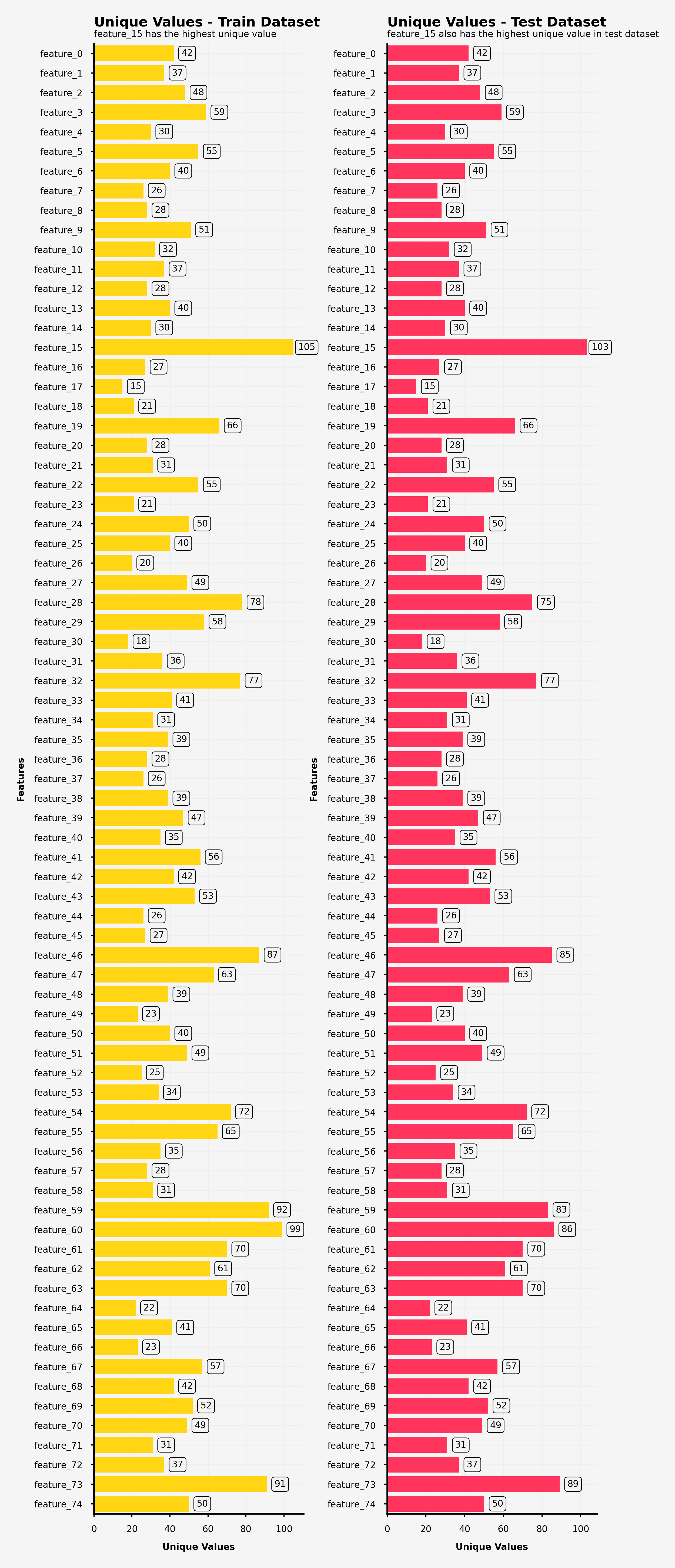
fig.patchesの部分複雑でした。
【可視化結果】
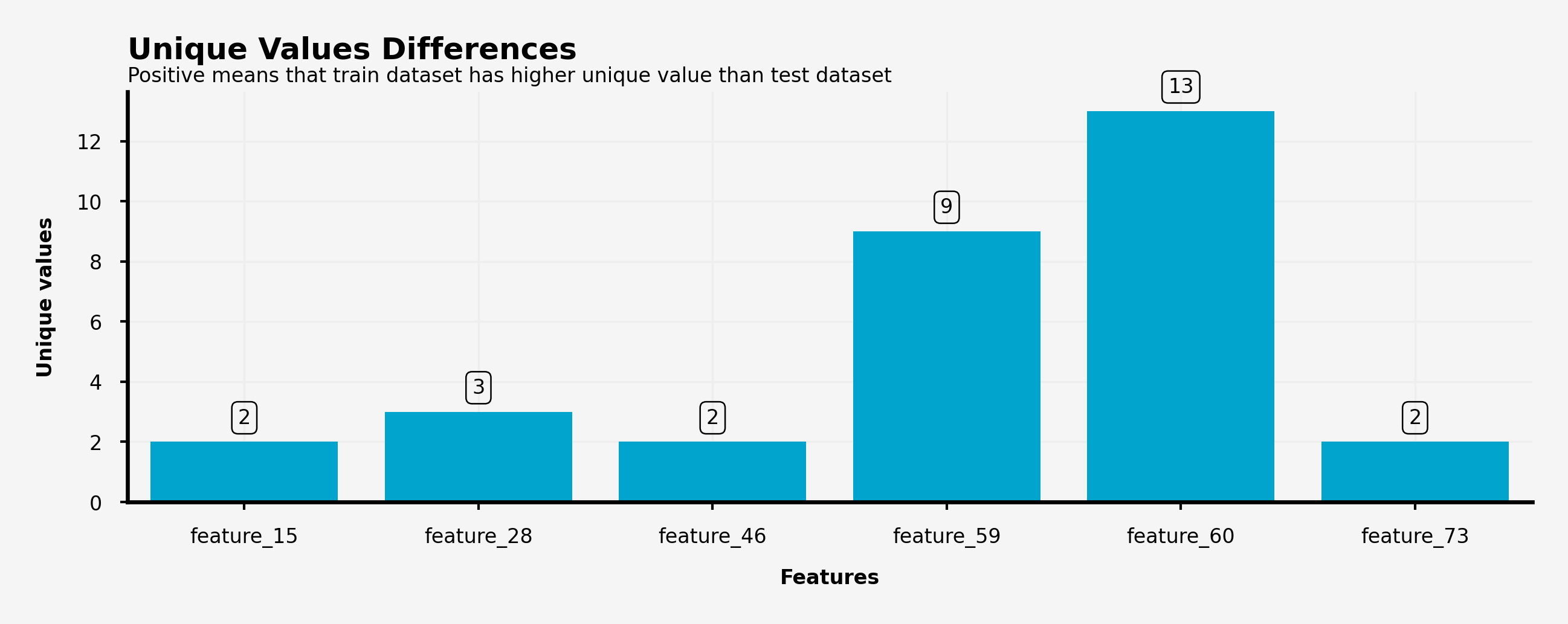
・feature_15がもっともユニークな特徴量の種類をもっており、以下feature_46, feature_59, feature_60 and feature_73が続く。
・feature_15, feature_28, feature_46, feature_59, feature_60 and feature_73は訓練データとテストデータで異なった特徴量の種類をもっており、feature_60は10種類も異なるユニークな特徴量を持つことになった。

以下二つ目の可視化結果についてグラフで表示しています。

plt.rcParams['figure.dpi'] = 600
fig = plt.figure(figsize=(5, 1.5), facecolor='#f6f5f5')
gs = fig.add_gridspec(1, 1)
gs.update(wspace=0.4, hspace=0.1)

background_color = "#f6f5f5"
sns.set_palette(['#00A4CCFF']*6)

ax = fig.add_subplot(gs[0, 0])
for s in ["right", "top"]:
    ax.spines[s].set_visible(False)
ax.set_facecolor(background_color)
ax_sns = sns.barplot(ax=ax, x=unique_value_feature_diff['Features'], 
                      y=unique_value_feature_diff['Count'], 
                      zorder=2, linewidth=0, alpha=1, saturation=1)
ax_sns.set_xlabel("Features",fontsize=4, weight='bold')
ax_sns.set_ylabel("Unique values",fontsize=4, weight='bold')
ax_sns.grid(which='major', axis='x', zorder=0, color='#EEEEEE', linewidth=0.4)
ax_sns.grid(which='major', axis='y', zorder=0, color='#EEEEEE', linewidth=0.4)
ax_sns.tick_params(labelsize=4, width=0.5, length=1.5)
ax.text(-0.5, 15.5, 'Unique Values Differences', fontsize=6, ha='left', va='top', weight='bold')
ax.text(-0.5, 14.5, 'Positive means that train dataset has higher unique value than test dataset', fontsize=4, ha='left', va='top')
# data label
for p in ax.patches:
    percentage = f'{p.get_height():.0f}'
    x = p.get_x() + p.get_width() / 2
    y = p.get_height() + 0.8
    ax.text(x, y, percentage, ha='center', va='center', fontsize=4,
           bbox=dict(facecolor='none', edgecolor='black', boxstyle='round', linewidth=0.3))

plt.show()

個々の特徴量における値の可視化

基本的にグラフの可視化については固定化されてるので、新出のものがあれば軽く解説します

mean_unique_value_train = pd.DataFrame(transpose_features_train.mean(axis=0))
# 全出現する特徴量の平均を算出
mean_unique_value_train = mean_unique_value_train.reset_index(drop=False) # インデックスの振り直し(0~141に)
mean_unique_value_train.columns = ['Unique', 'Mean'] # カラムの付与
mean_unique_value_train = mean_unique_value_train.sort_values('Mean', ascending=False)[:10] # 平均値について降順に
mean_unique_value_train

plt.rcParams['figure.dpi'] = 600
fig = plt.figure(figsize=(5, 1.5), facecolor='#f6f5f5')
gs = fig.add_gridspec(1, 1)
gs.update(wspace=0.4, hspace=0.1)

background_color = "#f6f5f5"
sns.set_palette(['#ffd514']*10)

ax = fig.add_subplot(gs[0, 0])
for s in ["right", "top"]:
    ax.spines[s].set_visible(False)
ax.set_facecolor(background_color)
ax_sns = sns.barplot(ax=ax, x=mean_unique_value_train['Unique'], 
                      y=mean_unique_value_train['Mean'], 
                      zorder=2, linewidth=0, alpha=1, saturation=1)
ax_sns.set_xlabel("Unique values",fontsize=4, weight='bold')
ax_sns.set_ylabel("Mean occurance",fontsize=4, weight='bold')
ax_sns.grid(which='major', axis='x', zorder=0, color='#EEEEEE', linewidth=0.4)
ax_sns.grid(which='major', axis='y', zorder=0, color='#EEEEEE', linewidth=0.4)
ax_sns.tick_params(labelsize=4, width=0.5, length=1.5)
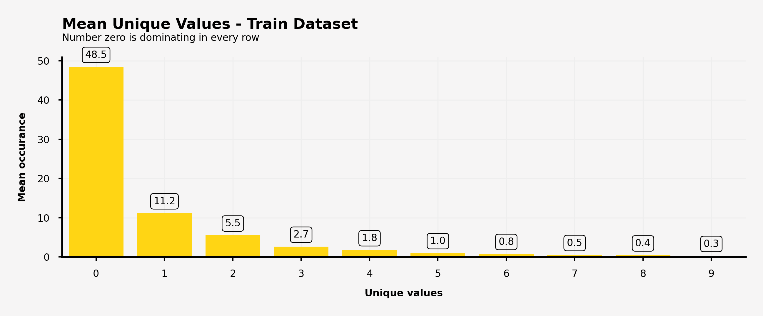
ax.text(-0.5, 61, 'Mean Unique Values - Train Dataset', fontsize=6, ha='left', va='top', weight='bold')
ax.text(-0.5, 57, 'Number zero is dominating in every row', fontsize=4, ha='left', va='top')
# data label
for p in ax.patches:
    percentage = f'{p.get_height():.1f}'
    x = p.get_x() + p.get_width() / 2
    y = p.get_height() + 3
    ax.text(x, y, percentage, ha='center', va='center', fontsize=4,
           bbox=dict(facecolor='none', edgecolor='black', boxstyle='round', linewidth=0.3))

plt.show()

mean_unique_value_test = pd.DataFrame(transpose_features_test.mean(axis=0))
mean_unique_value_test = mean_unique_value_test.reset_index(drop=False)
mean_unique_value_test.columns = ['Unique', 'Mean']
mean_unique_value_test = mean_unique_value_test.sort_values('Mean', ascending=False)[:10]
mean_unique_value_test

plt.rcParams['figure.dpi'] = 600
fig = plt.figure(figsize=(5, 1.5), facecolor='#f6f5f5')
gs = fig.add_gridspec(1, 1)
gs.update(wspace=0.4, hspace=0.1)

background_color = "#f6f5f5"
sns.set_palette(['#ff355d']*10)

ax = fig.add_subplot(gs[0, 0])
for s in ["right", "top"]:
    ax.spines[s].set_visible(False)
ax.set_facecolor(background_color)
ax_sns = sns.barplot(ax=ax, x=mean_unique_value_test['Unique'], 
                      y=mean_unique_value_test['Mean'], 
                      zorder=2, linewidth=0, alpha=1, saturation=1)
ax_sns.set_xlabel("Unique values",fontsize=4, weight='bold')
ax_sns.set_ylabel("Mean occurance",fontsize=4, weight='bold')
ax_sns.grid(which='major', axis='x', zorder=0, color='#EEEEEE', linewidth=0.4)
ax_sns.grid(which='major', axis='y', zorder=0, color='#EEEEEE', linewidth=0.4)
ax_sns.tick_params(labelsize=4, width=0.5, length=1.5)
ax.text(-0.5, 61, 'Mean Unique Values - Test Dataset', fontsize=6, ha='left', va='top', weight='bold')
ax.text(-0.5, 57, 'Number zero is dominating in every row', fontsize=4, ha='left', va='top')
# data label
for p in ax.patches:
    percentage = f'{p.get_height():.1f}'
    x = p.get_x() + p.get_width() / 2
    y = p.get_height() + 3
    ax.text(x, y, percentage, ha='center', va='center', fontsize=4,
           bbox=dict(facecolor='none', edgecolor='black', boxstyle='round', linewidth=0.3))

plt.show()

【可視化結果】
・特徴量の値0が最も訓練データセットとテストデータセットともに出現している。
・各値の出現率は0から始まる高い出現率の降順
・上位10個の出現率のデータから、訓練データとテストデータは同じ出現率の傾向を示している。

**** ０とそうではない値の分布の可視化

zero_positive_train = pd.DataFrame()
zero_positive_train['zero'] = transpose_features_train.iloc[:, 0]
zero_positive_train['positive'] = transpose_features_train.iloc[:,1:].sum(axis=1)

zero_positive_test = pd.DataFrame()
zero_positive_test['zero'] = transpose_features_test.iloc[:, 0]
zero_positive_test['positive'] = transpose_features_test.iloc[:,1:].sum(axis=1)

plt.rcParams['figure.dpi'] = 600
fig = plt.figure(figsize=(5, 2), facecolor='#f6f5f5')
gs = fig.add_gridspec(2, 1)
gs.update(wspace=0.4, hspace=1)

background_color = "#f6f5f5"
sns.set_palette(['#00A4CCFF'])

ax0 = fig.add_subplot(gs[0, 0])
for s in ["right", "top"]:
    ax0.spines[s].set_visible(False)
ax0.set_facecolor(background_color)
ax0_sns = sns.histplot(ax=ax0, x=zero_positive_train['positive'], zorder=2, color='#ff5573', linewidth=0.4, alpha=0.9)
ax0_sns = sns.histplot(ax=ax0, x=zero_positive_train['zero'], zorder=2, linewidth=0.4, alpha=0.9)
ax0_sns.set_xlabel("#No of occurance",fontsize=4, weight='bold')
ax0_sns.tick_params(labelsize=4, width=0.5, length=1.5)
ax0.text(-4, 8250, 'Train Dataset ', fontsize=6, ha='left', va='top', weight='bold')
ax0.text(-4, 7250, 'Zero has a higher occurance compare to positive numbers in train dataset', fontsize=4, ha='left', va='top')
ax0_sns.legend(['Positive', 'Zero'], ncol=2, facecolor=background_color, edgecolor=background_color, fontsize=3, bbox_to_anchor=(-0.01, 1.2), loc='upper left')
ax0_sns.set_ylabel("Count",fontsize=4, weight='bold')
ax0_sns.grid(which='major', axis='x', zorder=0, color='#EEEEEE', linewidth=0.4)
ax0_sns.grid(which='major', axis='y', zorder=0, color='#EEEEEE', linewidth=0.4)

ax1 = fig.add_subplot(gs[1, 0])
for s in ["right", "top"]:
    ax1.spines[s].set_visible(False)
ax1.set_facecolor(background_color)
ax1_sns = sns.histplot(ax=ax1, x=zero_positive_test['positive'], zorder=2, color='#ff5573', linewidth=0.4, alpha=0.9)
ax1_sns = sns.histplot(ax=ax1, x=zero_positive_test['zero'], zorder=2, linewidth=0.4, alpha=0.9)
ax1_sns.set_xlabel("#No of occurance",fontsize=4, weight='bold')
ax1_sns.tick_params(labelsize=4, width=0.5, length=1.5)
ax1.text(-4, 4250, 'Test Dataset ', fontsize=6, ha='left', va='top', weight='bold')
ax1.text(-4, 3700, 'Zero is also have a higher occurance compare to positive numbers in test dataset', fontsize=4, ha='left', va='top')
ax1_sns.legend(['Positive', 'Zero'], ncol=2, facecolor=background_color, edgecolor=background_color, fontsize=3, bbox_to_anchor=(-0.01, 1.2), loc='upper left')
ax1_sns.set_ylabel("Count",fontsize=4, weight='bold')
ax1_sns.grid(which='major', axis='x', zorder=0, color='#EEEEEE', linewidth=0.4)
ax1_sns.grid(which='major', axis='y', zorder=0, color='#EEEEEE', linewidth=0.4)

plt.show()

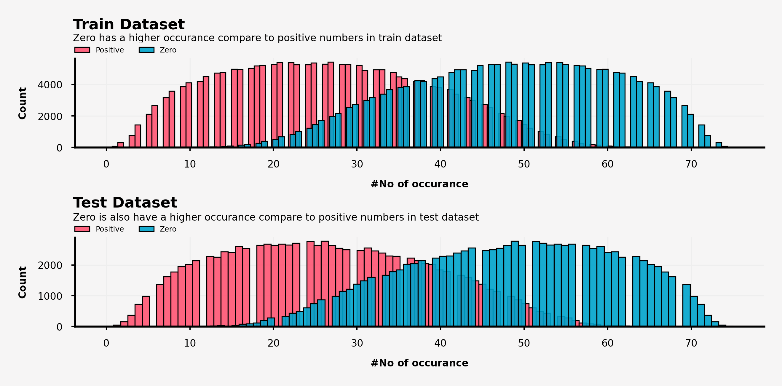
　何してるかというと、あるデータに対して0とそうではない数でそれぞれカウントして(合計は総特徴量の個数である75)、それぞれの数を棒グラフで可視化したものになります。

【可視化結果】
・訓練データとテストデータ両方において0はそうではない数より多く出現しており、まったく正反対の分布をとっている(=和が75になるため)。
・0とそうではない数の出現は訓練データとテストデータの間で違いが生じている。

　一見当たり前のようにしかみえない分布ですが、今回は0が多く出現していたためわかりやすかっただけだと思います。もし0ではなく本当にランダムに値が分散されている場合はこうした可視化を行わないとはっきりとデータの内容を掴めないような気がします。ただ、おそらくそのようなデータはまれで、今回のデータが特徴について何も説明がない完全にブラックボックスの状態で提供されていたためこうした議論に至ったと思います。

各特徴量における0~5の特徴量の頻度の可視化

　結構長くなりますのでなんとなくで見ていただければよいです。
　以下、同じようなコードが続くので変更箇所だけ 「# ← 変更」と明記します。

plt.rcParams['figure.dpi'] = 600
fig = plt.figure(figsize=(10, 10), facecolor='#f6f5f5')
gs = fig.add_gridspec(5, 5)
gs.update(wspace=0.3, hspace=0.3)

background_color = "#f6f5f5"
sns.set_palette(['#ffd514']*25)    # ← 変更  #ff355d

run_no = 0
for row in range(0, 5):
    for col in range(0, 5):
        locals()["ax"+str(run_no)] = fig.add_subplot(gs[row, col])
        locals()["ax"+str(run_no)].set_facecolor(background_color)
        for s in ["top","right"]:
            locals()["ax"+str(run_no)].spines[s].set_visible(False)
        run_no += 1

ax0.text(-0.5, 92, 'Top 5 Values - Train Dataset', fontsize=10, fontweight='bold')
ax0.text(-0.5, 85, 'features_0 - features_24', fontsize=6, fontweight='light')        

features = list(train_df.columns[1:26])    # ← 変更  train→test, 1:26→　27:52 → 53:75

run_no = 0
for col in features:
    temp_df = pd.DataFrame(train_df[col].value_counts())[:5]
    temp_df = temp_df.reset_index(drop=False)
    temp_df.columns = ['Number', 'Count']
    sns.barplot(ax=locals()["ax"+str(run_no)],x=temp_df['Number'], y=temp_df['Count']/len(train_df)*100, zorder=2, linewidth=0, alpha=1, saturation=1)    # ← 変更 train→test
    locals()["ax"+str(run_no)].grid(which='major', axis='x', zorder=0, color='#EEEEEE', linewidth=0.4)
    locals()["ax"+str(run_no)].grid(which='major', axis='y', zorder=0, color='#EEEEEE', linewidth=0.4)
    locals()["ax"+str(run_no)].set_ylabel('')
    locals()["ax"+str(run_no)].set_xlabel(col, fontsize=4, fontweight='bold')
    locals()["ax"+str(run_no)].tick_params(labelsize=4, width=0.5, length=1.5)
    locals()["ax"+str(run_no)].yaxis.set_major_formatter(ticker.PercentFormatter())
    # data label
    for p in locals()["ax"+str(run_no)].patches:
        percentage = f'{p.get_height():.1f}%\n'
        x = p.get_x() + p.get_width() / 2
        y = p.get_height()
        locals()["ax"+str(run_no)].text(x, y, percentage, ha='center', va='center', fontsize=4)

    run_no += 1

plt.show()

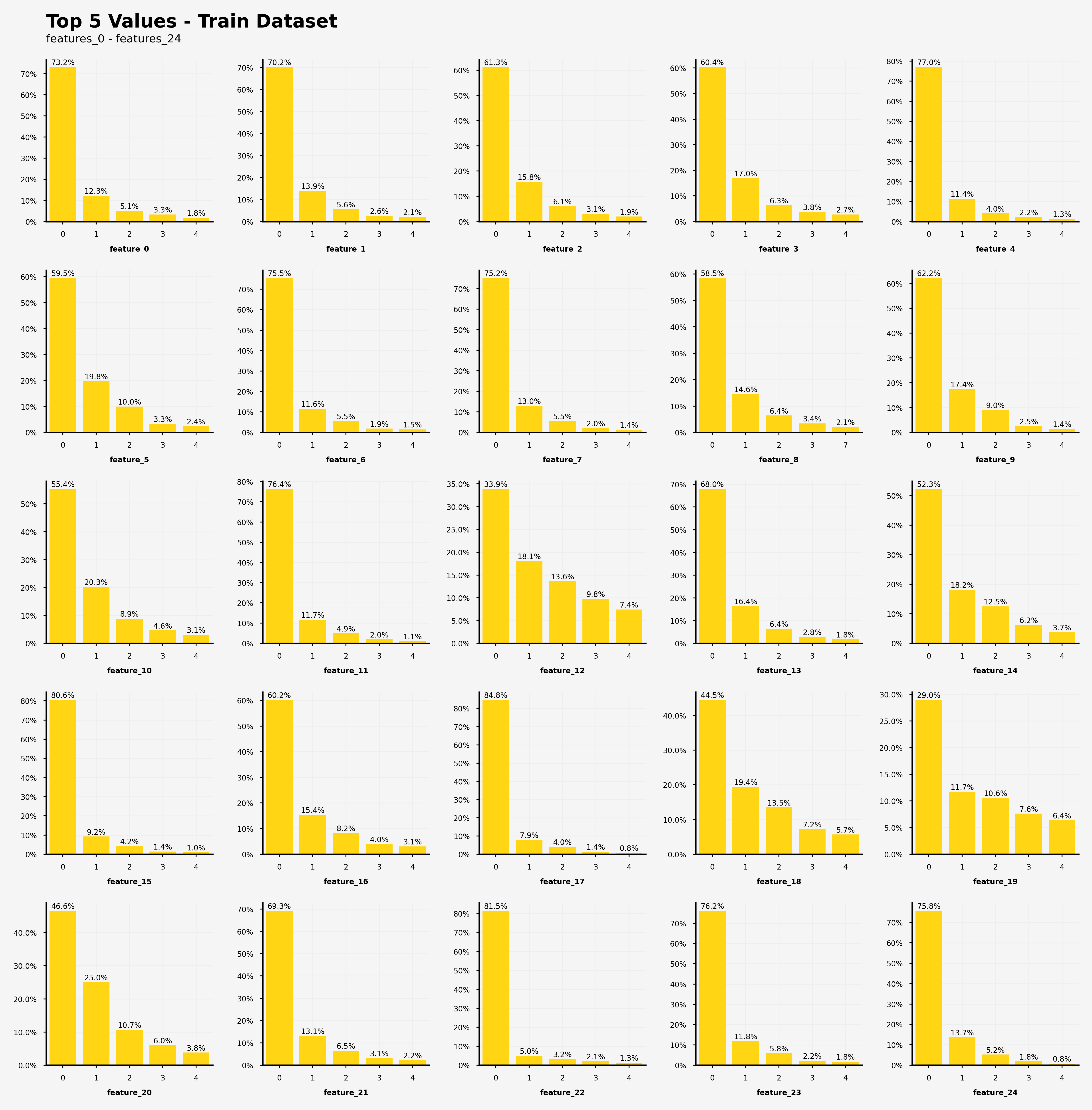
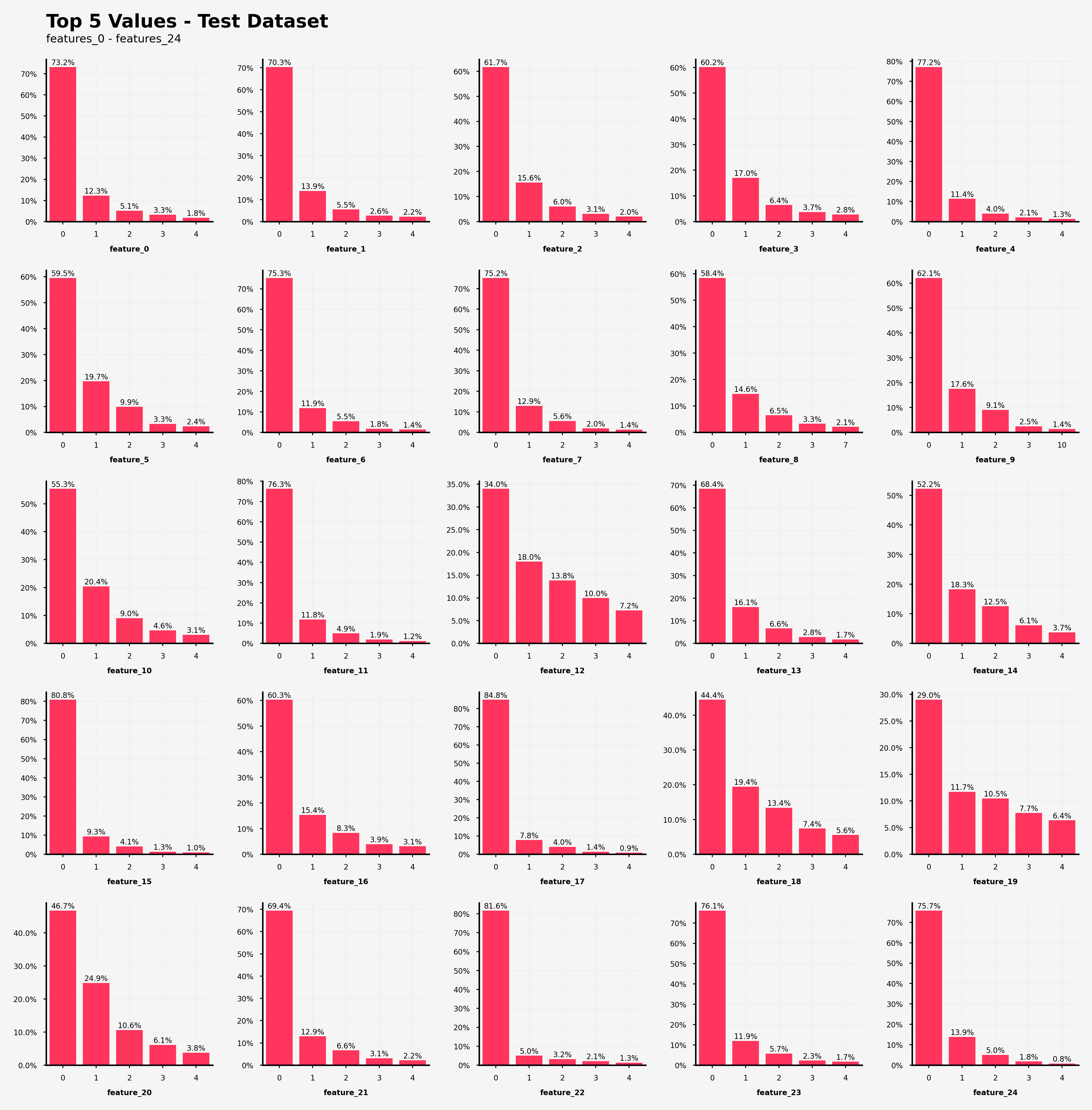
【訓練データにおける特徴0~24の特徴量の出現回数の可視化結果】
・feature_12, feature_18, feature_19, feature_20では0が支配的な特徴量の値(閾値50%)ではない
・feature_19だけ、上位5つの特徴量の値の出現率の総和が80%を上回っていない(=他の特徴量がfeature_19を説明している。)

【訓練データにおける特徴25~49の特徴量の出現回数の可視化結果】
・feature_31, feature_39, feature_43では0が支配的な特徴量の値(閾値50%)ではない
・feature_43だけ、上位5つの特徴量の値の出現率の総和が80%を上回っていない(=他の特徴量がfeature_43を説明している。)

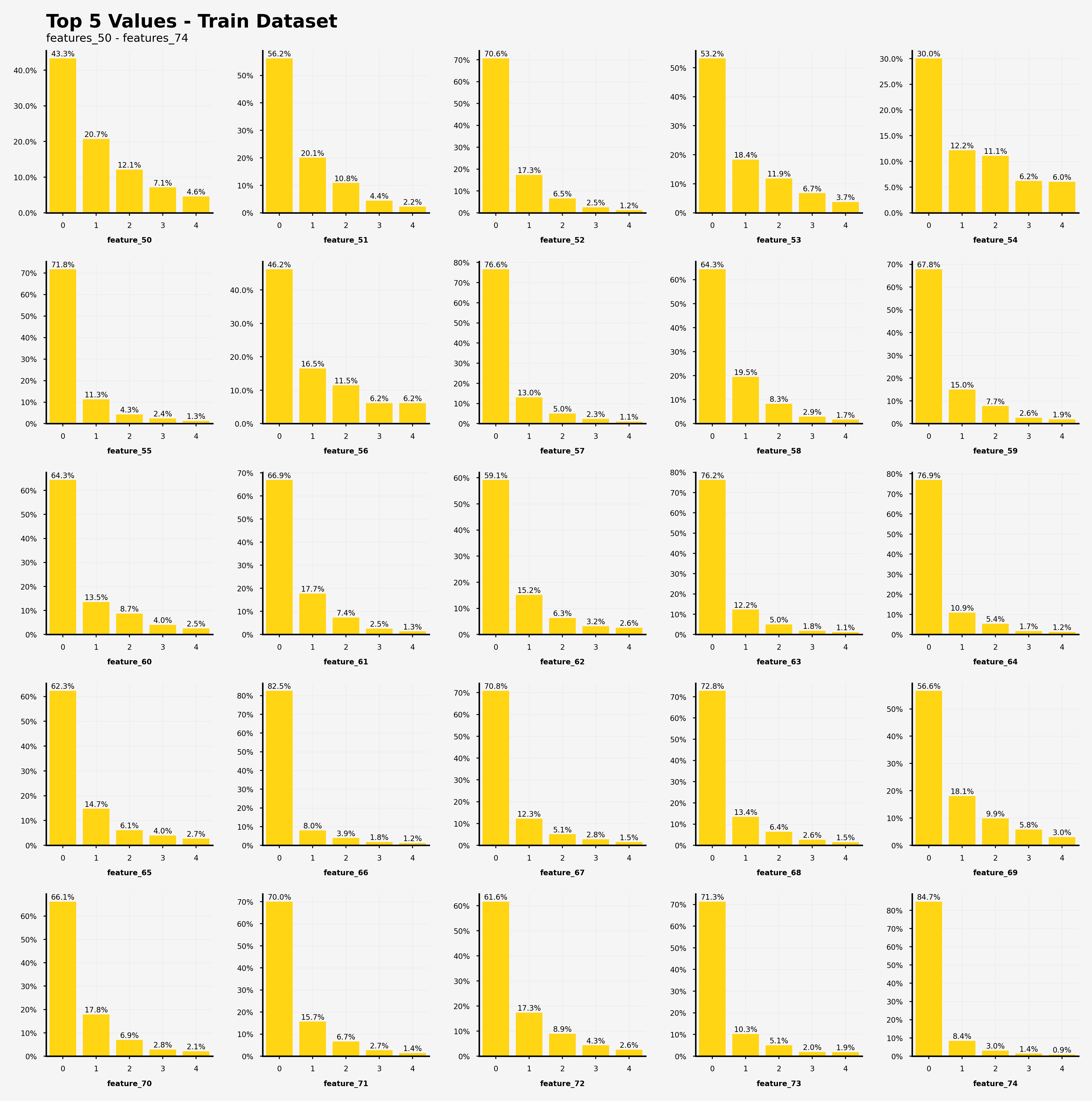
【訓練データにおける特徴50~74の特徴量の出現回数の可視化結果】
・feature_50, feature_54, feature_56では0が支配的な特徴量の値(閾値50%)ではない
・feature_54だけ、上位5つの特徴量の値の出現率の総和が80%を上回っていない(=他の特徴量がfeature_54を説明している。)

【テストデータにおける特徴25~49の特徴量の出現回数の可視化結果】
・feature_12, feature_18, feature_19, feature_20では0が支配的な特徴量の値(閾値50%)ではない
・feature_19だけ、上位5つの特徴量の値の出現率の総和が80%を上回っていない(=他の特徴量がfeature_19を説明している。)

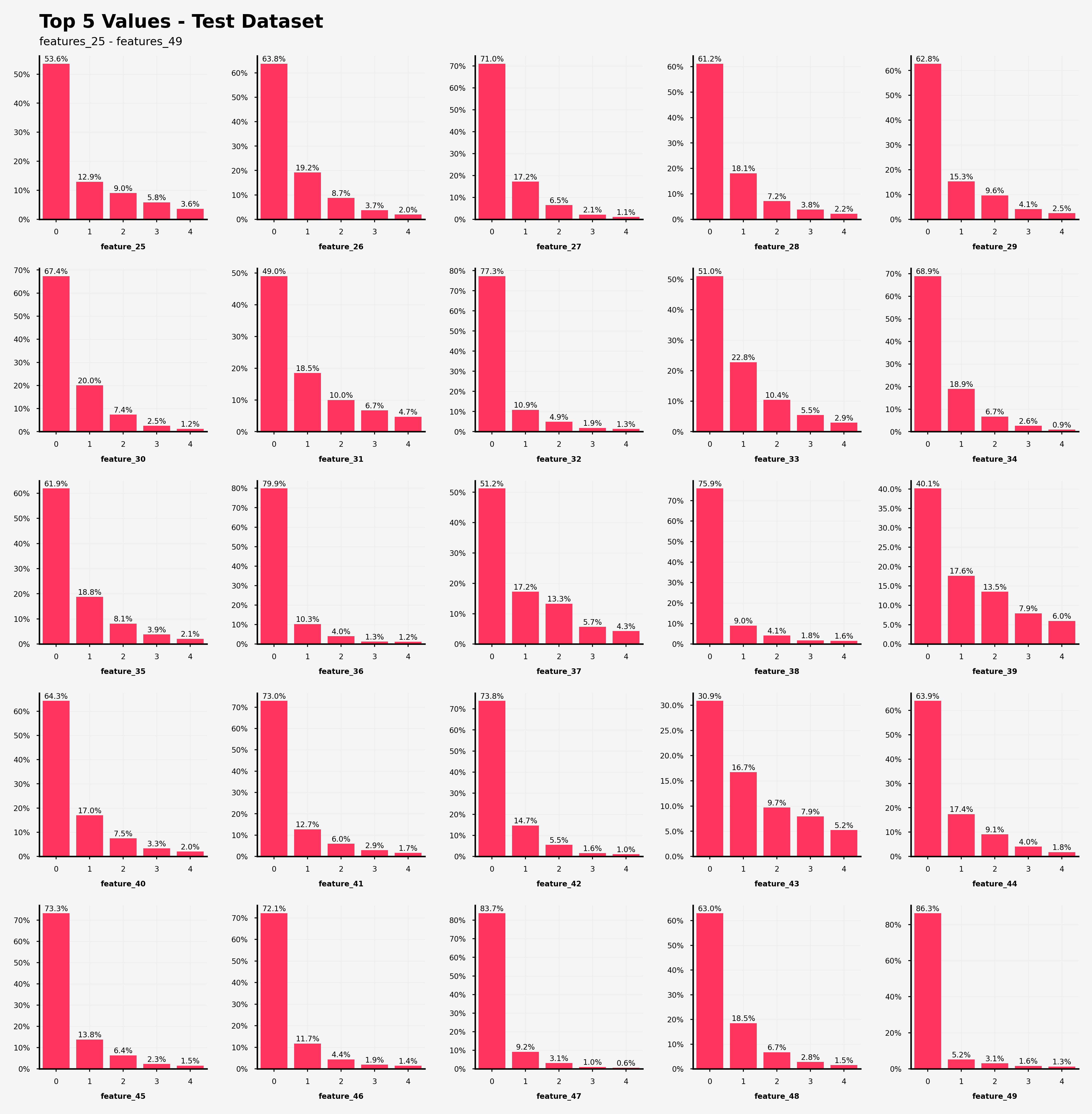
【テストデータにおける特徴25~49の特徴量の出現回数の可視化結果】
・feature_31, feature_39, feature_43では0が支配的な特徴量の値(閾値50%)ではない
・feature_43だけ、上位5つの特徴量の値の出現率の総和が80%を上回っていない(=他の特徴量がfeature_43を説明している。)

【テストデータにおける特徴50~74の特徴量の出現回数の可視化結果】
・feature_50, feature_54, feature_56では0が支配的な特徴量の値(閾値50%)ではない
・feature_54だけ、上位5つの特徴量の値の出現率の総和が80%を上回っていない(=他の特徴量がfeature_54を説明している。)

打ってて気づいたのですが、訓練データとテストデータを書き換えるだけでよく、つまり訓練データととテストデータのそれぞれの特徴量の出現頻度は全く同じでした。このコンペのあとに実際のデータの詳細が判明されれば面白かったりするのですが...

[TPS-Jun] This is Original EDA & VIZ

参考:[TPS-Jun] This is Original EDA & VIZ 😉

データの読み込み

import numpy as np
import pandas as pd
import matplotlib as mpl
import matplotlib.pyplot as plt
import seaborn as sns

# matplotlib setting
mpl.rcParams['figure.dpi'] = 200
mpl.rcParams['axes.spines.top'] = False
mpl.rcParams['axes.spines.right'] = False

train = pd.read_csv('train.csv')
test = pd.read_csv('test.csv')
sample_submission = pd.read_csv('sample_submission.csv')
train = train.drop('id', axis=1) # 後から追記しました(忘れてました)
test = test.drop('id', axis=1)

train.describe()
train.describe().T.style.bar(subset=['mean'], color='#205ff2').background_gradient(subset=['std'], cmap='Reds').background_gradient(subset=['50%'], cmap='coolwarm')
# T ... 転置。行と列の入れ替え。

pandasのデータフレームの変換が以下のサイトを参考にするといいと思います。
pandas – テーブルの表示をカスタマイズする方法
別に可視化する必要もないしおしゃれ程度ですよね...

データの確認

欠損値の確認

import missingno as msno

fig, ax = plt.subplots(1, 2, figsize=(20, 5))

msno.matrix(train, ax=ax[0], sparkline=False)
msno.matrix(test, ax=ax[1], sparkline=False)

ax[0].set_title('Train Null Data Check (0)', fontweight='bold')
ax[1].set_title('Test Null Data Check (0)', fontweight='bold')
plt.show()

こういう手法もあるらしいですけど、欠損値がないので何してるかさっぱりです。大学教授の安〇さんに怒られそうです。

目標変数の確認

fig = plt.figure(figsize=(12, 8))
gs = fig.add_gridspec(7, 4)
ax = fig.add_subplot(gs[:-1,:])
ax2 = fig.add_subplot(gs[-1,:])
ax2.axis('off')

target_cnt = train['target'].value_counts().sort_index()  # target変数の中のClass_の出現数をカウントし、Class_の名前でソートしている。(Class_1, Cass_2,...)
target_cum = target_cnt.cumsum() # 累積和、なくても支障はなかった...
ax.bar(target_cnt.index, target_cnt, color=['#d4dddd' if i%2==0 else '#fafafa' for i in range(9)],
       width=0.55, 
       edgecolor='black', 
       linewidth=0.7)


for i in range(9):
    ax.annotate(f'{target_cnt[i]}({target_cnt[i]/len(train)*100:.3}%)', xy=(i, target_cnt[i]+1000),
                   va='center', ha='center', # 中央に注釈が来るようにしている。vertical, horizontal 
               ) # ax.annoteta ...指定した位置(xy=())に注釈を入れる
    # 横棒グラフ
    ax2.barh([0], [target_cnt[i]], left=[target_cum[i] - target_cnt[i]], height=0.2, 
            edgecolor='black', linewidth=0.7, color='#d4dddd' if i%2==0 else '#fafafa'
            )
    ax2.annotate(i+1, xy=(target_cum[i]-target_cnt[i]/2, 0), 
                 va='center', ha='center', fontsize=10)

ax.set_title('Target Distribution', weight='bold', fontsize=15)
ax.grid(axis='y', linestyle='-', alpha=0.4)

fig.tight_layout()
plt.show()

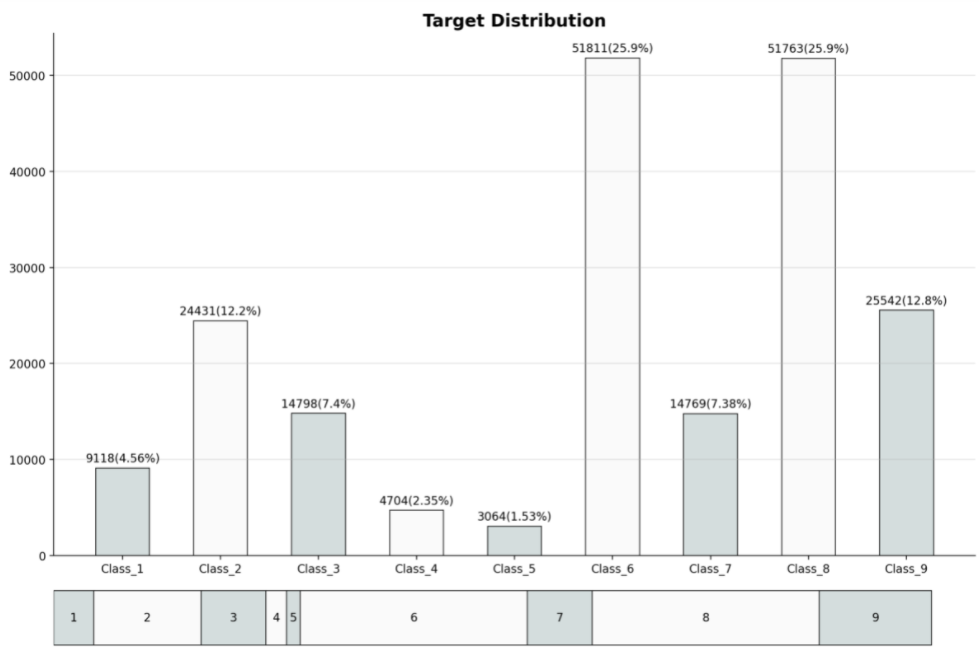
　どちらの方もadd_gridspecを用いてる...カテゴリカル変数の出現回数をカウントしているだけですが、かなり目標変数の分布についての理解が深まったと思います。結構役にたつ可視化手法な気がする。

target_cnt_df = pd.DataFrame(target_cnt)
target_cnt_df['ratio(%)'] = target_cnt_df/target_cnt.sum()*100
target_cnt_df.sort_values('ratio(%)', ascending=False, inplace=True)
target_cnt_df['cummulated_sum(%)'] = target_cnt_df['ratio(%)'].cumsum()
target_cnt_df

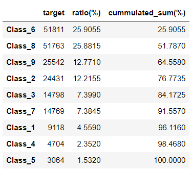
　上の図から上位４クラスでデータの75%を占めてることがわかります。

　それぞれの特徴量のユニークな数について調べて、訓練データとテストデータのユニークな数の違いを調べる

説明変数の確認

　訓練データとテストデータで出現する特徴量の違い

# １つ目の図
fig, ax = plt.subplots(1, 1, figsize=(15, 6))

# train[].nuniqueでユニークな特徴量の数を取り出し、それを全特徴量分(75)調べてる。
y = np.array([train[f'feature_{i}'].nunique() for i in range(75)])
y2 = np.array([test[f'feature_{i}'].nunique() for i in range(75)])
comp = y-y2

# barの引数でrange()みたいな使い方できるんですね...
ax.bar(range(75), y2, alpha=0.7, color='lightgray', label='Test Dataset')
ax.bar(range(75),  comp*(comp>0), bottom=y2, color='#336666', alpha=0.7, label='Train > Test')
ax.bar(range(75), comp*(comp<0), bottom=y2-comp*(comp<0), color='#e3120b', alpha=0.7, label='Train < Test')

ax.set_yticks(range(0, 110, 5))
ax.set_xticks(range(0, 75, 5))
ax.margins(0.01)
ax.grid(axis='y', linestyle='--', zorder=5)
ax.set_title('# of Features Unique Values (Train/Test)', loc='left', fontweight='bold')
ax.legend()
plt.show()



# 二つ目の図
pd.DataFrame(data={'feature' : np.arange(75)[comp>0], 
              'delta' : comp[comp>0]}, index=None)

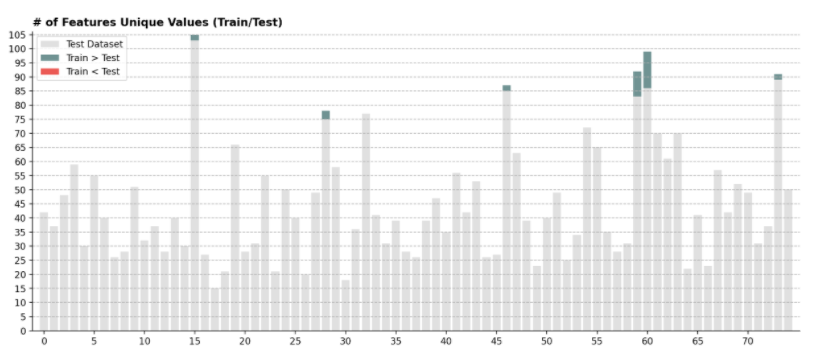
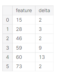
　テストデータより訓練データの方がユニークな特徴量が多いことがわかります。

　特徴量の平均

test_mean = test.mean()
idx = np.argsort(test_mean)

train_mean = train.mean()[idx]
test_mean = test_mean.sort_values()

comp = train_mean-test_mean

fig, ax = plt.subplots(1, 1, figsize=(15, 6))

ax.bar(range(75), test_mean, alpha=0.7, color='lightgray', label='Test Dataset')
ax.bar(range(75),  comp*(comp>0), bottom=test_mean, color='#336666', alpha=0.7, label='Train > Test')
ax.bar(range(75), comp*(comp<0), bottom=test_mean-comp*(comp<0), color='#e3120b', alpha=0.7, label='Train < Test')

ax.margins(0.01)
ax.grid(axis='y', linestyle='--', zorder=5)
ax.set_title('Mean of Features (Sorted by Test)', loc='left', fontweight='bold')
ax.legend()
plt.show()

　訓練データとテストデータにおける特徴量の平均に差分が生じていたら緑or赤で色づけられます。平均に大きな差がみられないあたり、各特徴量の値の出現回数は訓練データとテストデータともにほぼ同じであるといっていいでしょう。

クラスごとの特徴量の平均と全体の特徴量の平均の違いの可視化

fig, axes = plt.subplots(3, 3, figsize=(15, 12))

train_mean = train.mean().sort_values() # 全体のへ雨域ん
mean_idx = np.argsort(train.mean())
axes = axes.flatten()

for idx, target_feature in enumerate(sorted(train['target'].unique())): # 目的変数Class_1, ...9)について
    sub_mean = train[train['target']==target_feature].mean()[mean_idx]
    comp = train_mean-sub_mean

    ax = axes[idx]
    ax.bar(range(75), sub_mean, alpha=0.7, color='lightgray')
    ax.bar(range(75),  comp*(comp>0), bottom=sub_mean, color='#336666', alpha=0.7, label=f'Train > {target_feature}')
    ax.bar(range(75), comp*(comp<0), bottom=sub_mean-comp*(comp<0), color='#e3120b', alpha=0.7, label=f'Train < {target_feature}')

    ax.margins(0.01)
    ax.set_xticks([])
    ax.set_yticks([])
    ax.set_title(f'{target_feature}', fontweight='bold', loc='left', bbox=dict(boxstyle='round', fc="#efe8d1", ec="k"))
    ax.spines['left'].set_visible(False)
    ax.legend(fontsize=8)

fig.supxlabel('Average by class (by Class)', ha='center', fontweight='bold')    
plt.show()

クラス2とか3では全体の特徴に比べてやや低い値で出現してることがわかります。

特徴量毎の各クラスにおける平均の可視化

fig, axes = plt.subplots(15, 5, figsize=(10, 20))

target_order = sorted(train['target'].unique())
mean = train.groupby('target').mean().sort_index()
std = train.groupby('target').std().sort_index()

for idx, ax in zip(range(75), axes.flatten()):
    ax.bar(mean[f'feature_{idx}'].index, mean[f'feature_{idx}'], 
           color=['#efe8d1' if i%2==0 else '#acc8d4' for i in range(9)],
           edgecolor='black', 
           linewidth=0.4,
           width=0.6)
    
    ax.set_xticks([])
    ax.set_yticks([])
    ax.set_xlabel('')
    ax.set_ylabel('')
    ax.margins(0.1)
    ax.spines['left'].set_visible(False)
    ax.set_title(f'Feature_{idx}', loc='right', weight='bold', fontsize=10)

fig.supxlabel('Average by class (by feature)', ha='center', fontweight='bold')

fig.tight_layout()
plt.show()

各説明変数の分布の可視化

0の割合を調べる

fig, ax = plt.subplots(1, 1, figsize=(15, 6))

ax.bar(range(75), 100, linewidth=0.2, edgecolor='black', alpha=0.2, color='lightgray')
ax.bar(range(75), ((train == 0).sum() / len(train)*100)[:-1].sort_values(), linewidth=0.2, edgecolor='black', alpha=1, color='#244747')

ax.set_ylim(0, 100)
ax.set_yticks(range(0, 100, 10))

ax.set_xticks(range(0, 75, 5))
ax.margins(0.01)
ax.grid(axis='y', linestyle='--', linewidth=0.2, zorder=5)
ax.set_title('Ratio of Zeros (Sorted)', loc='center', fontweight='bold')
ax.set_ylabel('ratio(%)', fontsize=12)
ax.legend()
plt.show()

　経緯としては特徴量の大部分が0のため、これを可視化しようという感じ(らしい)です。

【可視化結果】
・0の割合は各特徴量ごとに30～80まで幅広く分布している。
・可視化してないけど、訓練データとテストデータともに0の割合の分布は同じようなものになるらしいです。

UMAPを使った次元削減

次元削減自体PCAくらいしか知らなかったので調べる価値ありそうです。後日記事にしても面白そうかも。Kaggleをしていると書籍には載っていない最新の手法が使われていたりするので(pyplyとか)やっててすごくためになります。
・最新の次元圧縮法"UMAP"について
・次元削減手法（まとめと実装）PCA, LSI(SVD), LDA, ICA, PLIS

label_dict = {val:idx for idx, val in enumerate(sorted(train['target'].unique()))}
# print(label_dict)
train['target'] = train['target'].map(label_dict)
# データ0~199999とそれに対応するクラス1~9を紐づけている。

pip install umap-learn 
%%time
from umap import UMAP

train_sub = train.sample(50000, random_state=72)
target = train_sub['target']
umap = UMAP(random_state=0)
dr = umap.fit_transform(train_sub.iloc[:,:-1], target)

カラーパレットの作成

# https://www.kaggle.com/subinium/dark-mode-visualization-apple-version
light_palette = [
    (0, 122, 255), # Blue
    (255, 149, 0), # Orange
    (52, 199, 89), # Green
    (255, 59, 48), # Red
    (175, 82, 222),# Purple
    (255, 45, 85), # Pink
    (88, 86, 214), # Indigo
    (90, 200, 250),# Teal
    (255, 204, 0)  # Yellow
]

fig = plt.figure(figsize=(20, 20))
gs = fig.add_gridspec(10, 9)
ax = fig.add_subplot(gs[:-1,:])

sub_axes = [None] * 9
for idx in range(9): 
    sub_axes[idx] = fig.add_subplot(gs[-1,idx])

for idx in range(9):
    ax.scatter(x=dr[:,0][target==idx], y=dr[:,1][target==idx],
              s=10, alpha=0.2
              )

    for j in range(9):
        sub_axes[j].scatter(x=dr[:,0][target==idx], y=dr[:,1][target==idx],
                            s=10, alpha = 0.4 if idx==j else 0.008, 
                            color = '#%02x%02x%02x' % light_palette[j] if idx==j else 'gray',
                            zorder=(idx==j)
                           )
        
    
    sub_axes[idx].set_xticks([])
    sub_axes[idx].set_yticks([])
    sub_axes[idx].set_xlabel('')
    sub_axes[idx].set_ylabel('')
    sub_axes[idx].set_title(f'Class_{idx+1}')
    sub_axes[idx].spines['right'].set_visible(True)
    sub_axes[idx].spines['top'].set_visible(True)

ax.set_title('Dimenstion Reduction (UMAP)', fontweight='bold', fontfamily='serif', fontsize=20, loc='left')   
    
ax.set_xticks([])
ax.set_yticks([])
ax.set_xlabel('')
ax.set_ylabel('')
ax.spines['left'].set_visible(False)
ax.spines['bottom'].set_visible(False)

fig.tight_layout()
plt.show()

%%time
test_sub = train.sample(50000, random_state=72)
dr_test = umap.transform(test_sub)

import matplotlib.patches as mpatches


fig, ax = plt.subplots(1, 1, figsize=(20, 20))
ax.scatter(x=dr[:,0], y=dr[:,1], 
           color = '#%02x%02x%02x' % light_palette[0],
           s=10, alpha=0.3, label='Train')
ax.scatter(x=dr_test[:,0], y=dr_test[:,1], 
           color = '#%02x%02x%02x' % light_palette[1],
           s=10, alpha=0.3, label='Test')


ax.set_title('Dimenstion Reduction Compare (Train/Test)', fontweight='bold', fontfamily='serif', fontsize=20, loc='left')   
    
ax.set_xticks([])
ax.set_yticks([])
ax.set_xlabel('')
ax.set_ylabel('')
ax.spines['left'].set_visible(False)
ax.spines['bottom'].set_visible(False)

train_dot = mpatches.Patch(color='#%02x%02x%02x' % light_palette[0], label='Train')
test_dot = mpatches.Patch(color='#%02x%02x%02x' % light_palette[1], label='Train')
ax.legend(handles=[train_dot, test_dot], loc='lower center', ncol = 2, fontsize=15)
fig.tight_layout()
plt.show()

　正直可視化結果についてはわかりにくかったですが、モデル構築の際に次元圧縮とかも考慮できたら面白そうです。

⚡Catboost with Optuna Starter [TPS-06]

参考:⚡Catboost with Optuna Starter [TPS-06]
本記事では勾配ブースティング決定木の一つであるCatboostを用いてデータの予測を行っています。実装の記事に関してはDay3でとりあげるつもりで、Day2では行った可視化についてまとめます。

データの可視化

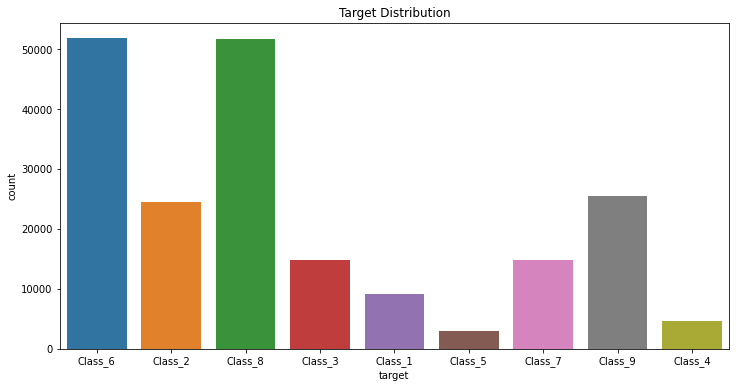
目標変数の出現回数を棒グラフで表現

fig, ax = plt.subplots(figsize=(12, 6))
sns.countplot(x='target', data=train)
ax.set_title('Target Distribution')

pandasのtableを使った可視化

train.drop(columns=['id']).describe().T.style.bar(subset=['mean'], color='#606ff2')\
                            .background_gradient(subset=['std'], cmap='PuBu')\
                            .background_gradient(subset=['50%'], cmap='PuBu')
# testについても同様のことを行ってました。

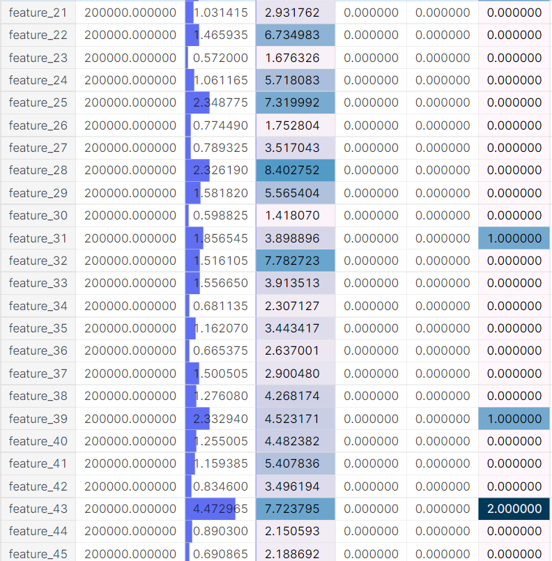
よく調べなかったのもあるのですが、事前の可視化はここまででした。

おわりに

今週中にモデルを取り扱った記事を出そうと思います。